Pl Please run & analyze the data and provide the work.

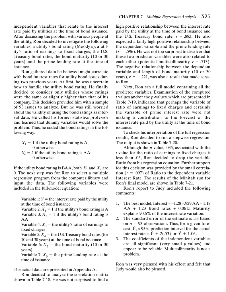
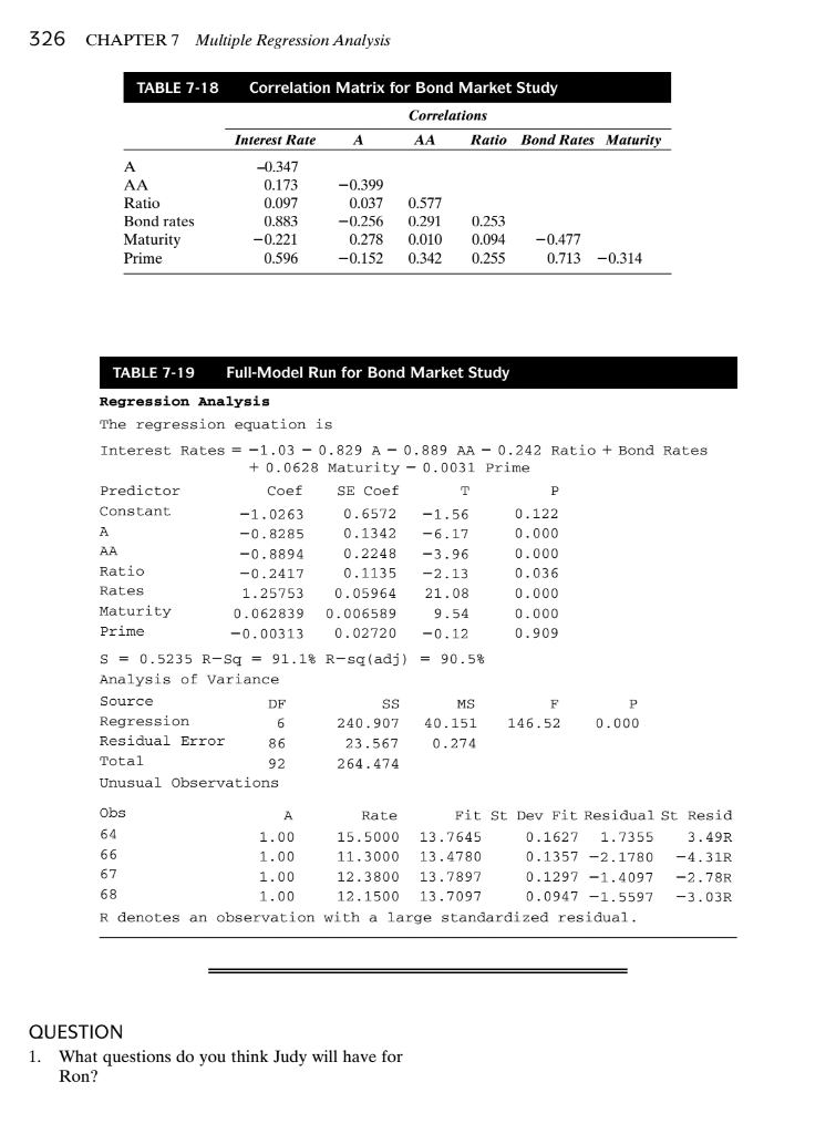
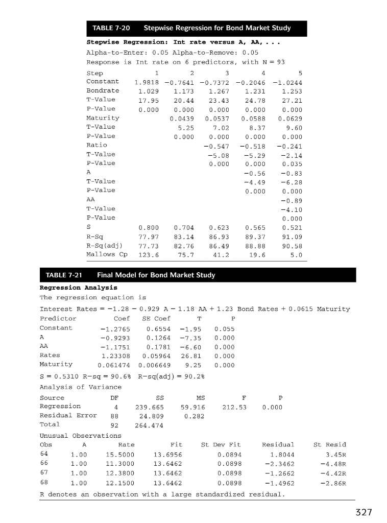
CASES CASE 7-1 THE BOND MARKET16 Judy Johnson, vice president of finance of a large, private, investor-owned utility in the Northwest, was faced with a financing problem. The company needed money both to pay off short-term debts coming due and to continue construction of a coal- fired plant. Judy's main concern was estimating the 10- or 30-year bond market; the any needed to decide whether to use equity financing or long-term debt. To make this decision, the utility needed a reliable forecast of the interest rate it would pay at the time of bond issuance. Judy called a meeting of her financial staff to discuss the bond market problem. One member of her staff, Ron Peterson, a recent M.B.A. graduate, said he thought a multiple regression model could be developed to forecast the bond rates. Since the vice president was not familiar with multiple regres- sion, she steered the discussion in another direction. After an hour of unproductive interaction, Judy then asked Ron to have a report on her desk the fol- lowing Monday. Ron knew that the key to the development of a good forecasting model is the identification of 16 The data for this case study were provided by Dorothy Mercer, an Eastern Washington University M.B.A. student. The analysis was done by M.B.A. students Tak Fu, Ron Hand, Dorothy Mercer, Mary Lou Redmond, and Harold Wilson. CHAPTER 7 Multiple Regression Analysis 325 independent variables that relate to the interest rate paid by utilities at the time of bond issuance. After discussing the problem with various people at the utility, Ron decided to investigate the following variables: a utility's bond rating (Moody's), a util- ity's ratio of earnings to fixed charges, the U.S. Treasury bond rates, the bond maturity (10 or 30 years), and the prime lending rate at the time of issuance. Ron gathered data he believed might correlate with bond interest rates for utility bond issues dur- ing two previous years. At first, he was uncertain how to handle the utility bond rating. He finally decided to consider only utilities whose ratings were the same or slightly higher than that of his company. This decision provided him with a sample of 93 issues to analyze. But he was still worried about the validity of using the bond ratings as inter- val data. He called his former statistics professor and learned that dummy variables would solve the problem. Thus, he coded the bond ratings in the fol- lowing way: high positive relationship between the interest rate paid by the utility at the time of bond issuance and the U.S. Treasury bond rate, r = .883. He also expected a fairly high positive relationship between the dependent variable and the prime lending rate (r = .596). He was not too surprised to discover that these two predictor variables were also related to each other (potential multicollinearity, r = .713). The negative relationship between the dependent variable and length of bond maturity (10 or 30 years), r = -221, was also a result that made sense to Ron. Next, Ron ran a full model containing all the predictor variables. Examination of the computed t values and/or the p-values, which are presented in Table 7-19, indicated that perhaps the variable of ratio of earnings to fixed charges and certainly the variable of prime interest rate were not making a contribution to the forecast of the interest rate paid by the utility at the time of bond issuance. To check his interpretation of the full regression results, Ron decided to run a stepwise regression. The output is shown in Table 7-20. Although the p-value, .035, associated with the I value for the ratio of earnings to fixed charges is less than .05, Ron decided to drop the variable Ratio from his regression equation. Further support for this decision was provided by the small correla- tion (r = .097) of Ratio to the dependent variable Interest Rate. The results of the Minitab run for Ron's final model are shown in Table 7-21. Ron's report to Judy included the following comments: X1 = 1 if the utility bond rating is A; 0 otherwise X2 = 1 if the utility bond rating is AA; 0 otherwise If the utility bond rating is BAA, both X, and X2 are 0. The next step was for Ron to select a multiple regression program from the computer library and input the data. The following variables were included in the full-model equation: Variable 1: Y = the interest rate paid by the utility at the time of bond issuance Variable 2: X, = 1 if the utility's bond rating is A Variable 3: X2 = 1 if the utility's bond rating is AA Variable 4: X2 = the utility's ratio of earnings to fixed charges Variable 5: X4 = the U.S. Treasury bond rates (for 10 and 30 years) at the time of bond issuance Variable 6: X, = the bond maturity (10 or 30 years) Variable 7: X6 = the prime lending rate at the time of issuance 1. The best model, Interest =-1.28 -929 AA-1.18 AA + 1.23 Bond rates + 0.0615 Maturity, explains 90.6% of the interest rate variation. 2. The standard error of the estimate is .53 based on n = 93 observations. Thus, for a given fore- cast, Y, a 95% prediction interval for the actual interest rate is 20.53) or + 1.06. 3. The coefficients of the independent variables are all significant (very small p-values) and appear to be reliable. Multicollinearity is not a problem. Ron was very pleased with his effort and felt that Judy would also be pleased. The actual data are presented in Appendix A. Ron decided to analyze the correlation matrix shown in Table 7-18. He was not surprised to find a 326 CHAPTER 7 Multiple Regression Analysis TABLE 7-18 A AA Ratio Bond rates Maturity Prime Correlation Matrix for Bond Market Study Correlations Interest Rate AA Ratio Bond Rates Maturity -0.347 0.173 -0.399 0.097 0.037 0.577 0.883 -0.256 0.291 0.253 0.010 0,094 -0.477 0.596 -0.152 0.342 0.713 -0.314 -0.221 0.278 0.255 TABLE 7-19 Full-Model Run for Bond Market Study Regression Analysis The regression equation is Interest Rates = -1.03 - 0.829 A-0.889 AA -0.242 Ratio + Bond Rates + 0.0628 Maturity -0.0031 Prime Predictor Coef SE Coef T P Constant -1.0263 0.6572 -1.56 0.122 A -0.8285 0.1342 -6.17 0.000 AA -0.8894 0.2248 -3.96 0.000 Ratio -0.2417 0.1135 -2.13 0.036 Rates 1.25753 0.05964 21.08 0.000 Maturity 0.062839 0.006589 9.54 0.000 Prime -0.00313 0.02720 -0.12 0.909 S = 0.5235 R-Sq = 91.1% R-sq(adj) = 90.5% Analysis of Variance Source DF SS MS F P Regression 6 240.907 40.151 146.52 0.000 Residual Error 86 23.567 0.274 Total 92 264.474 Unusual Observations Obs A Rate Fit St Dev Fit Residual St Resid 64 1.00 15.5000 13.7645 0.1627 1.7355 3.49R 66 1.00 11.3000 13.4780 0.1357 -2.1780 -4.31R 67 1.00 12.3800 13.7897 0.1297 -1.4097 -2.78R 68 1.00 12.1500 13.7097 0.0947 -1.5597 -3.03R R denotes an observation with a large standardized residual. QUESTION 1. What questions do you think Judy will have for Ron? TABLE 7-20 Stepwise Regression for Bond Market Study Stepwise Regression: Int rate versus A, AA, ... Alpha-to-Enter: 0.05 Alpha-to-Remove: 0.05 Response is Int rate on 6 predictors, with N = 93 Step 1 2 3 4 5 Constant 1.9818 -0.7641 -0.7372 -0.2046 -1.0244 Bondrate 1.029 1.173 1.267 1.231 1.253 T-Value 17.95 20.44 23.43 24.78 27.21 P-Value 0.000 0.000 0.000 0.000 0.000 Maturity 0.0439 0.0537 0.0588 0.0629 T-Value 5.25 7.02 8.37 9.60 P-Value 0.000 0.000 0.000 0.000 Ratio -0.547 -0.518 -0.241 T-Value - -5.08 -5.29 -2.14 P-Value P 0.000 0.000 0.035 A -0.56 -0.83 T-Value -4.49 -6.28 P-Value 0.000 0.000 AA -0.89 T-Value -4.10 P-Value 0.000 S 0.800 0.704 0.623 0.565 0.521 R-S 77.97 83.14 86.93 89.37 91.09 R-Sq(adj) 77.73 82.76 86.49 88.88 90.58 Mallows Cp 123.6 75.7 41.2 19.6 5.0 = TABLE 7-21 Final Model for Bond Market Study Regression Analysis The regression equation is Interest Rates = -1.28 - 0.929 A-1.18 AA + 1.23 Bond Rates + 0.0615 Maturity Predictor Coef SE Coef P Constant -1.2765 0.6554 -1.95 0.055 A A -0.9293 0.1264 -7.35 0.000 AA -1.1751 0.1781 -6.60 0.000 Rates 1.23308 0.05964 26.81 0.000 Maturity 0.061474 0.006649 9.25 0.000 S = 0.5310 R-sq = 90.6% R-sq(adj) = 90.2% Analysis of variance Source DF SS MS F P Regression 4 239.665 59.916 212.53 0.000 Residual Error 88 24.809 0.282 Total 92 264.474 Unusual Observations Obs A Rate Fit St Dev Fit Residual St Resid 64 1.00 15.5000 13.6956 0.0894 1.8044 3.45R 66 1.00 11.3000 13.6462 0.0898 -2.3462 -4.48R 67 1.00 12.3800 13.6462 0.0898 -1.2662 -4.42R 68 1.00 12.1500 13.6462 0.0898 -1.4962 -2.86R R denotes an observation with a large standardized residual. 327