Please answer Q2/Q3 and show the python code with a picture as well

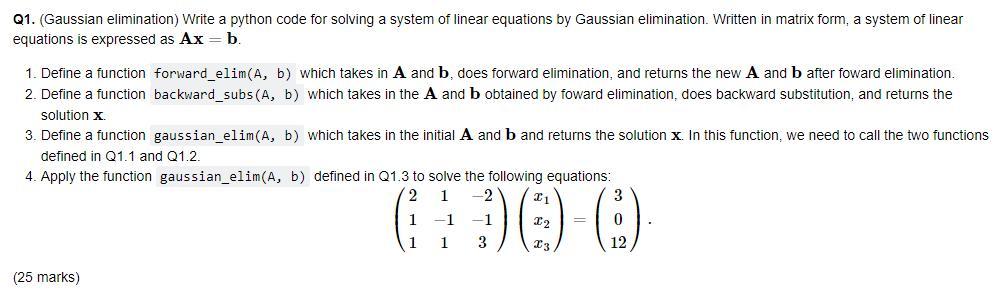
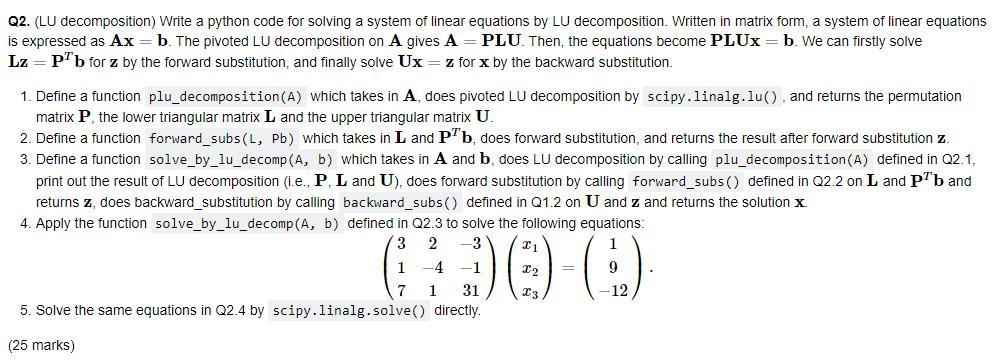
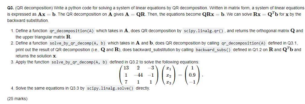
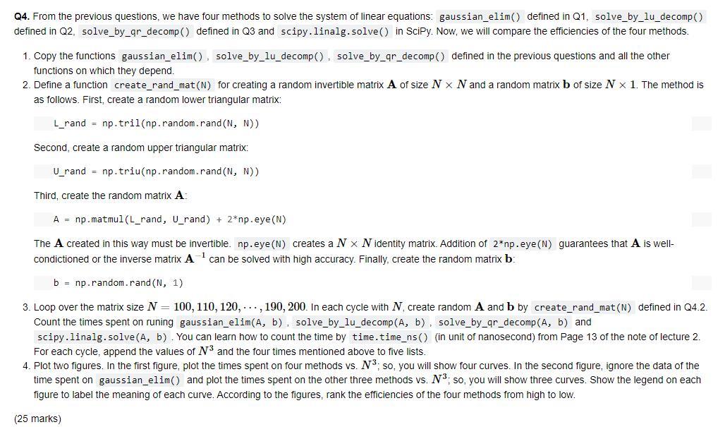
Q1. (Gaussian elimination) Write a python code for solving a system of linear equations by Gaussian elimination. Written in matrix form, a system of linear equations is expressed as Ax=b. 1. Define a function forward_elim(A, b) which takes in A and b, does forward elimination, and returns the new A and b after foward elimination. 2. Define a function backward_subs(A, b) which takes in the A and b obtained by foward elimination, does backward substitution, and returns the solution x. 3. Define a function gaussian_elim(a, b) which takes in the initial A and b and returns the solution x. In this function, we need to call the two functions defined in Q1.1 and 21.2. 4. Apply the function gaussian_elim(A, b) defined in Q1.3 to solve the following equations: 2 2 (3 1) ) -(0) (25 marks) Q2. (LU decomposition) Write a python code for solving a system of linear equations by LU decomposition. Written in matrix form, a system of linear equations is expressed as Ax = b. The pivoted LU decomposition on A gives A PLU. Then, the equations become PLUx=b. We can firstly solve Lz = PTb for z by the forward substitution, and finally solve Ux = z for x by the backward substitution. 1. Define a function plu_decomposition(A) which takes in A, does pivoted LU decomposition by scipy.linalg.lu), and returns the permutation matrix P. the lower triangular matrix L and the upper triangular matrix U. 2. Define a function forward_subs(L, Pb) which takes in L and PTb, does forward substitution, and returns the result after forward substitution z. 3. Define a function solve_by_lu_decomp (A, b) which takes in A and b, does LU decomposition by calling plu_decomposition(A) defined in 22.1, print out the result of LU decomposition (i.e., P. L and U), does forward substitution by calling forward_subs() defined in Q2.2 on L and Pb and returns z, does backward_substitution by calling backward_subs() defined in Q1.2 on U and z and returns the solution x 4. Apply the function solve_by_lu_decomp (A, b) defined in Q2.3 to solve the following equations: 3 2 -3 21 1-4 -1 22 9 1 31 C3 12 5. Solve the same equations in Q2.4 by scipy.linalg.solve directly. (25 marks) Q3. (QR decomposition) Write a python code for solving a system of linear equations by QR decomposition. Written in matrix form, a system of linear equations is expressed as Ax=b. The QR decomposition on A gives A QR. Then, the equations become QRx b. We can solve Rx = Q'b for x by the backward substitution 1. Define a function qr_decomposition(A) which takes in A, does QR decomposition by scipy.linalg.qr(), and returns the orthogonal matrix Q and the upper triangular matrix R 2. Define a function solve_by_gr_decomp (A, b) which takes in A and b, does QR decomposition by calling gr_decomposition(A) defined in Q3.1, print out the result of QR decomposition (i.e., Q and R), does backward_substitution by calling backward_subs() defined in Q1.2 on R and Q'b and returns the solution x. 3. Apply the function solve_by_9r_decomp(A, b) defined in Q3.2 to solve the following equations: 13 2 3 1 -44 -1 22 0.9 7 1 4. Solve the same equations in 23.3 by scipy.linalg. solve directly. (25 marks) Q4. From the previous questions, we have four methods to solve the system of linear equations: gaussian_elim() defined in Q1, solve_by_lu_decomp) defined in Q2, solve_by_gr_decomp() defined in Q3 and scipy.linalg.solve()in SciPy. Now, we will compare the efficiencies of the four methods. 1. Copy the functions gaussian_elim(), solve_by_lu_decomp() solve_by_gr_decomp() defined in the previous questions and all the other functions on which they depend. 2. Define a function create_rand_mat(N) for creating a random invertible matrix A of size Nx N and a random matrix b of size N x 1. The method is as follows. First, create a random lower triangular matrix: L_rand = np.tril(np.random.rand(N, N)) Second, create a random upper triangular matrix U_rand = np.triu(np.random.rand(N, N)) Third, create the random matrix A: A = np.matmul(L_rand, U_rand) + 2*np.eye(N) The A created in this way must be invertible. np.eye(N) creates a N x N identity matrix. Addition of 2*np.eye(N) guarantees that A is well- condictioned or the inverse matrix Acan be solved with high accuracy. Finally, create the random matrix b b = np.random.rand (N, 1) 3. Loop over the matrix size N = 100, 110, 120, ..., 190, 200. In each cycle with N, create random A and b by create_rand_mat(N) defined in Q4.2. Count the times spent on runing gaussian_elim(A, b). solve_by_lu_decomp (A, b), solve_by_gr_decomp (A, b) and scipy.linalg. solve (A, b). You can learn how to count the time by time.time_ns() (in unit of nanosecond) from Page 13 of the note of lecture 2. For each cycle, append the values of N3 and the four times mentioned above to five lists. 4. Plot two figures. In the first figure, plot the times spent on four methods vs. N3: so, you will show four curves. In the second figure, ignore the data of the time spent on gaussian_elim() and plot the times spent on the other three methods vs. N3: so, you will show three curves. Show the legend on each figure to label the meaning of each curve. According to the figures, rank the efficiencies of the four methods from high to low. (25 marks) Q1. (Gaussian elimination) Write a python code for solving a system of linear equations by Gaussian elimination. Written in matrix form, a system of linear equations is expressed as Ax=b. 1. Define a function forward_elim(A, b) which takes in A and b, does forward elimination, and returns the new A and b after foward elimination. 2. Define a function backward_subs(A, b) which takes in the A and b obtained by foward elimination, does backward substitution, and returns the solution x. 3. Define a function gaussian_elim(a, b) which takes in the initial A and b and returns the solution x. In this function, we need to call the two functions defined in Q1.1 and 21.2. 4. Apply the function gaussian_elim(A, b) defined in Q1.3 to solve the following equations: 2 2 (3 1) ) -(0) (25 marks) Q2. (LU decomposition) Write a python code for solving a system of linear equations by LU decomposition. Written in matrix form, a system of linear equations is expressed as Ax = b. The pivoted LU decomposition on A gives A PLU. Then, the equations become PLUx=b. We can firstly solve Lz = PTb for z by the forward substitution, and finally solve Ux = z for x by the backward substitution. 1. Define a function plu_decomposition(A) which takes in A, does pivoted LU decomposition by scipy.linalg.lu), and returns the permutation matrix P. the lower triangular matrix L and the upper triangular matrix U. 2. Define a function forward_subs(L, Pb) which takes in L and PTb, does forward substitution, and returns the result after forward substitution z. 3. Define a function solve_by_lu_decomp (A, b) which takes in A and b, does LU decomposition by calling plu_decomposition(A) defined in 22.1, print out the result of LU decomposition (i.e., P. L and U), does forward substitution by calling forward_subs() defined in Q2.2 on L and Pb and returns z, does backward_substitution by calling backward_subs() defined in Q1.2 on U and z and returns the solution x 4. Apply the function solve_by_lu_decomp (A, b) defined in Q2.3 to solve the following equations: 3 2 -3 21 1-4 -1 22 9 1 31 C3 12 5. Solve the same equations in Q2.4 by scipy.linalg.solve directly. (25 marks) Q3. (QR decomposition) Write a python code for solving a system of linear equations by QR decomposition. Written in matrix form, a system of linear equations is expressed as Ax=b. The QR decomposition on A gives A QR. Then, the equations become QRx b. We can solve Rx = Q'b for x by the backward substitution 1. Define a function qr_decomposition(A) which takes in A, does QR decomposition by scipy.linalg.qr(), and returns the orthogonal matrix Q and the upper triangular matrix R 2. Define a function solve_by_gr_decomp (A, b) which takes in A and b, does QR decomposition by calling gr_decomposition(A) defined in Q3.1, print out the result of QR decomposition (i.e., Q and R), does backward_substitution by calling backward_subs() defined in Q1.2 on R and Q'b and returns the solution x. 3. Apply the function solve_by_9r_decomp(A, b) defined in Q3.2 to solve the following equations: 13 2 3 1 -44 -1 22 0.9 7 1 4. Solve the same equations in 23.3 by scipy.linalg. solve directly. (25 marks) Q4. From the previous questions, we have four methods to solve the system of linear equations: gaussian_elim() defined in Q1, solve_by_lu_decomp) defined in Q2, solve_by_gr_decomp() defined in Q3 and scipy.linalg.solve()in SciPy. Now, we will compare the efficiencies of the four methods. 1. Copy the functions gaussian_elim(), solve_by_lu_decomp() solve_by_gr_decomp() defined in the previous questions and all the other functions on which they depend. 2. Define a function create_rand_mat(N) for creating a random invertible matrix A of size Nx N and a random matrix b of size N x 1. The method is as follows. First, create a random lower triangular matrix: L_rand = np.tril(np.random.rand(N, N)) Second, create a random upper triangular matrix U_rand = np.triu(np.random.rand(N, N)) Third, create the random matrix A: A = np.matmul(L_rand, U_rand) + 2*np.eye(N) The A created in this way must be invertible. np.eye(N) creates a N x N identity matrix. Addition of 2*np.eye(N) guarantees that A is well- condictioned or the inverse matrix Acan be solved with high accuracy. Finally, create the random matrix b b = np.random.rand (N, 1) 3. Loop over the matrix size N = 100, 110, 120, ..., 190, 200. In each cycle with N, create random A and b by create_rand_mat(N) defined in Q4.2. Count the times spent on runing gaussian_elim(A, b). solve_by_lu_decomp (A, b), solve_by_gr_decomp (A, b) and scipy.linalg. solve (A, b). You can learn how to count the time by time.time_ns() (in unit of nanosecond) from Page 13 of the note of lecture 2. For each cycle, append the values of N3 and the four times mentioned above to five lists. 4. Plot two figures. In the first figure, plot the times spent on four methods vs. N3: so, you will show four curves. In the second figure, ignore the data of the time spent on gaussian_elim() and plot the times spent on the other three methods vs. N3: so, you will show three curves. Show the legend on each figure to label the meaning of each curve. According to the figures, rank the efficiencies of the four methods from high to low. (25 marks)