Please comment with email so I can send data thanks.

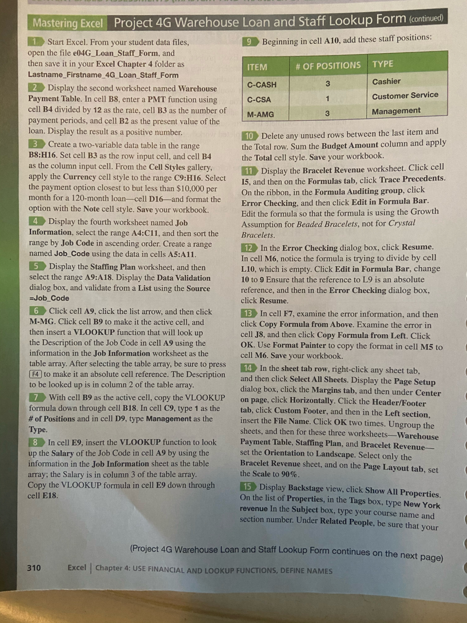
Mastering Excel Project 4G Warehouse Loan and Staff Lookup Form (continued) 1. Start Excel. From your student data files, 9 Beginning in cell A10, add these staff positions: open the file e04G_Loan_Staff_Form, and then save it in your Excel Chapter 4 folder as ITEM # OF POSITIONS TYPE Lastname_Firstname_4G Loan Staff Form Cashier 2 Display the second worksheet named Warehouse C-CASH Payment Table. In cell B8, enter a PMT function using C-CSA Customer Service cell B4 divided by 12 as the rate, cell B3 as the number of M-AMG Management payment periods, and cell B2 as the present value of the loan. Display the result as a positive number. 10 Delete any unused rows between the last item and 3 Create a two-variable data table in the range the Total row. Sum the Budget Amount column and apply B8:H16. Set cell B3 as the row input cell, and cell B4 the Total cell style. Save your workbook. as the column input cell. From the Cell Styles gallery, 11 Display the Bracelet Revenue worksheet. Click cell apply the Currency cell style to the range C9:H16. Select 15, and then on the Formulas tab, click Trace Precedents. the payment option closest to but less than $10,000 per On the ribbon, in the Formula Auditing group, click month for a 120-month loan-cell D16and format the Error Checking, and then click Edit in Formula Bar. option with the Note cell style. Save your workbook. Edit the formula so that the formula is using the Growth 4 Display the fourth worksheet named Job Assumption for Beaded Bracelets, not for Crystal Information, select the range A4:C11, and then sort the Bracelets. range by Job Code in ascending order. Create a range 12 In the Error Checking dialog box, click Resume. named Job_Code using the data in cells A5:A11. In cell M6, notice the formula is trying to divide by cell 5 Display the Staffing Plan worksheet, and then L10, which is empty. Click Edit in Formula Bar, change select the range A9:A18. Display the Data Validation 10 to 9 Ensure that the reference to L9 is an absolute dialog box, and validate from a List using the Source reference, and then in the Error Checking dialog box, =Job_Code click Resume. 6 Click cell A9, click the list arrow, and then click 13 In cell F7, examine the error information, and then M-MG. Click cell B9 to make it the active cell, and click Copy Formula from Above. Examine the error in then insert a VLOOKUP function that will look up cell J8, and then click Copy Formula from Left. Click the Description of the Job Code in cell A9 using the OK. Use Format Painter to copy the format in cell M5 to information in the Job Information worksheet as the cell M6. Save your workbook. table array. After selecting the table array, be sure to press 14 In the sheet tab row, right-click any sheet tab. (F4 to make it an absolute cell reference. The Description and then click Select All Sheets. Display the Page Setup to be looked up is in column 2 of the table array. dialog box, click the Margins tab, and then under Center 7 With cell B9 as the active cell, copy the VLOOKUP on page, click Horizontally. Click the Header/Footer formula down through cell B18. In cell C9, type 1 as the tab, click Custom Footer, and then in the Left section, # of Positions and in cell D9, type Management as the insert the File Name. Click OK two times. Ungroup the Type. sheets, and then for these three worksheets-Warehouse 8 In cell E9, insert the VLOOKUP function to look Payment Table, Staffing Plan, and Bracelet Revenue up the Salary of the Job Code in cell A9 by using the set the Orientation to Landscape. Select only the information in the Job Information sheet as the table Bracelet Revenue sheet, and on the Page Layout tab, set array; the Salary is in column 3 of the table array. the Scale to 90%. Copy the VLOOKUP formula in cell E9 down through 15 Display Backstage view, click Show All Properties. cell E18. On the list of Properties, in the Tags box, type New York revenue In the Subject box, type your course name and section number. Under Related People, be sure that your (Project 4G Warehouse Loan and Staff Lookup Form continues on the next 310 Excel Chapter 4: USE FINANCIAL AND LOOKUP FUNCTIONS, DEFINE NAMES Mastering Excel Project 4G Warehouse Loan and Staff Lookup Form (continued) 1. Start Excel. From your student data files, 9 Beginning in cell A10, add these staff positions: open the file e04G_Loan_Staff_Form, and then save it in your Excel Chapter 4 folder as ITEM # OF POSITIONS TYPE Lastname_Firstname_4G Loan Staff Form Cashier 2 Display the second worksheet named Warehouse C-CASH Payment Table. In cell B8, enter a PMT function using C-CSA Customer Service cell B4 divided by 12 as the rate, cell B3 as the number of M-AMG Management payment periods, and cell B2 as the present value of the loan. Display the result as a positive number. 10 Delete any unused rows between the last item and 3 Create a two-variable data table in the range the Total row. Sum the Budget Amount column and apply B8:H16. Set cell B3 as the row input cell, and cell B4 the Total cell style. Save your workbook. as the column input cell. From the Cell Styles gallery, 11 Display the Bracelet Revenue worksheet. Click cell apply the Currency cell style to the range C9:H16. Select 15, and then on the Formulas tab, click Trace Precedents. the payment option closest to but less than $10,000 per On the ribbon, in the Formula Auditing group, click month for a 120-month loan-cell D16and format the Error Checking, and then click Edit in Formula Bar. option with the Note cell style. Save your workbook. Edit the formula so that the formula is using the Growth 4 Display the fourth worksheet named Job Assumption for Beaded Bracelets, not for Crystal Information, select the range A4:C11, and then sort the Bracelets. range by Job Code in ascending order. Create a range 12 In the Error Checking dialog box, click Resume. named Job_Code using the data in cells A5:A11. In cell M6, notice the formula is trying to divide by cell 5 Display the Staffing Plan worksheet, and then L10, which is empty. Click Edit in Formula Bar, change select the range A9:A18. Display the Data Validation 10 to 9 Ensure that the reference to L9 is an absolute dialog box, and validate from a List using the Source reference, and then in the Error Checking dialog box, =Job_Code click Resume. 6 Click cell A9, click the list arrow, and then click 13 In cell F7, examine the error information, and then M-MG. Click cell B9 to make it the active cell, and click Copy Formula from Above. Examine the error in then insert a VLOOKUP function that will look up cell J8, and then click Copy Formula from Left. Click the Description of the Job Code in cell A9 using the OK. Use Format Painter to copy the format in cell M5 to information in the Job Information worksheet as the cell M6. Save your workbook. table array. After selecting the table array, be sure to press 14 In the sheet tab row, right-click any sheet tab. (F4 to make it an absolute cell reference. The Description and then click Select All Sheets. Display the Page Setup to be looked up is in column 2 of the table array. dialog box, click the Margins tab, and then under Center 7 With cell B9 as the active cell, copy the VLOOKUP on page, click Horizontally. Click the Header/Footer formula down through cell B18. In cell C9, type 1 as the tab, click Custom Footer, and then in the Left section, # of Positions and in cell D9, type Management as the insert the File Name. Click OK two times. Ungroup the Type. sheets, and then for these three worksheets-Warehouse 8 In cell E9, insert the VLOOKUP function to look Payment Table, Staffing Plan, and Bracelet Revenue up the Salary of the Job Code in cell A9 by using the set the Orientation to Landscape. Select only the information in the Job Information sheet as the table Bracelet Revenue sheet, and on the Page Layout tab, set array; the Salary is in column 3 of the table array. the Scale to 90%. Copy the VLOOKUP formula in cell E9 down through 15 Display Backstage view, click Show All Properties. cell E18. On the list of Properties, in the Tags box, type New York revenue In the Subject box, type your course name and section number. Under Related People, be sure that your (Project 4G Warehouse Loan and Staff Lookup Form continues on the next 310 Excel Chapter 4: USE FINANCIAL AND LOOKUP FUNCTIONS, DEFINE NAMES