Portfolio optimization with a risk-free asset

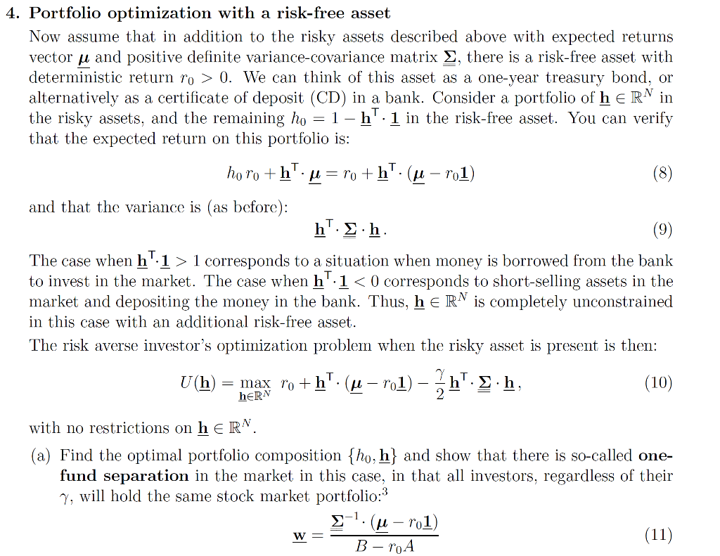
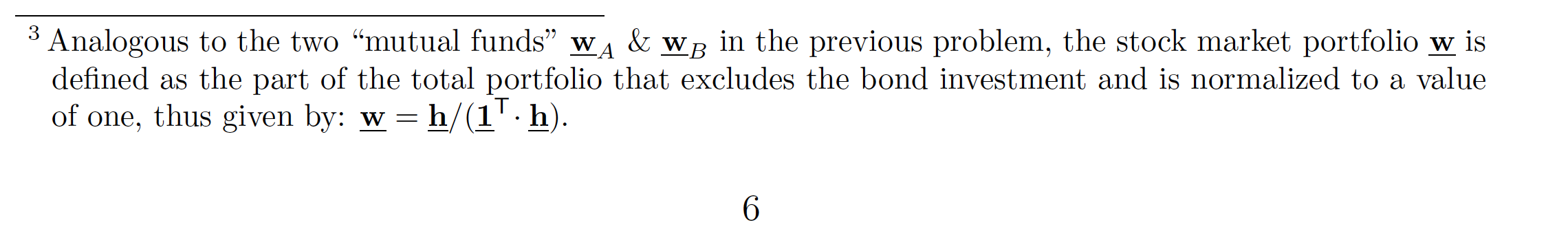
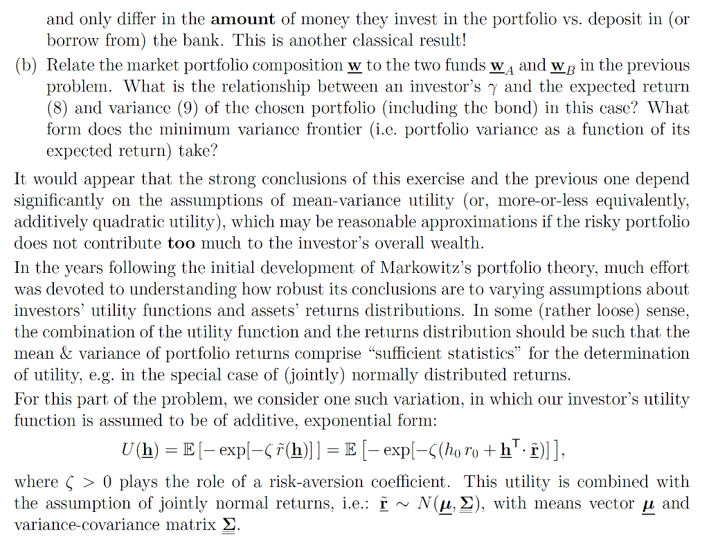
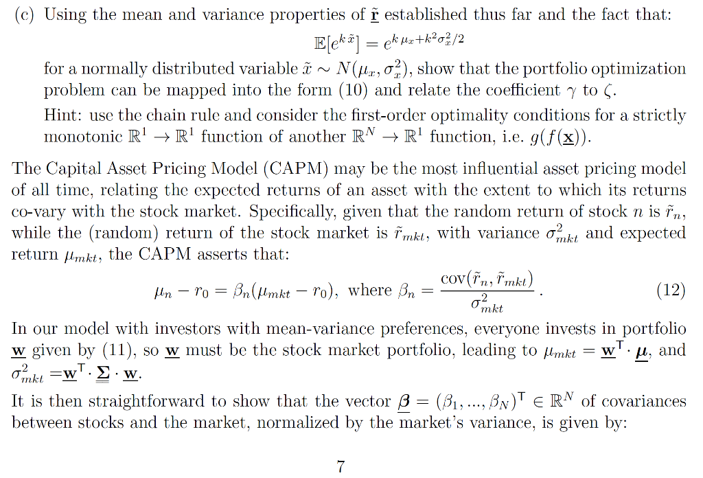
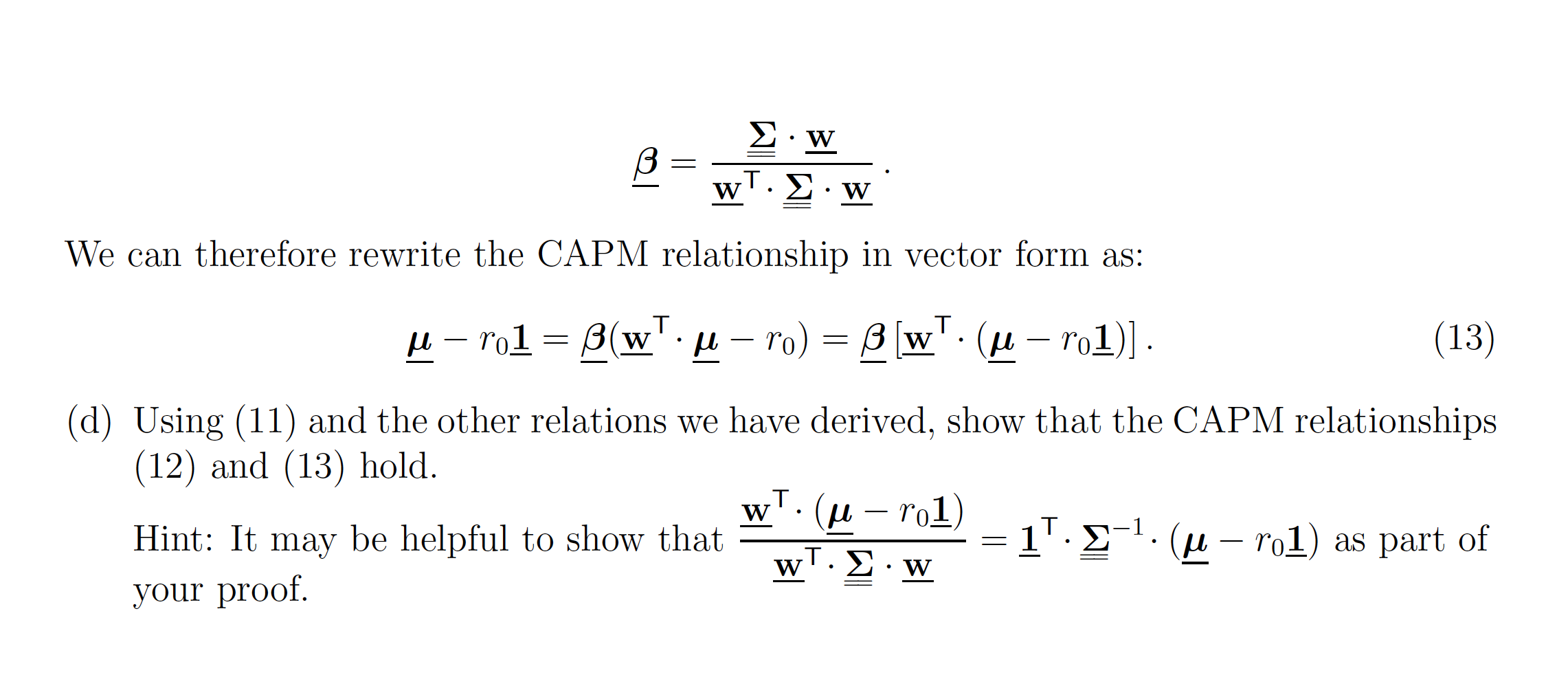
4. Portfolio optimization with a risk-free asset Now assume that in addition to the risky assets described above with expected returns vector u and positive definite variance-covariance matrix ?, there is a risk-free asset with deterministic return ro > 0. We can think of this asset as a one-year treasury bond, or alternatively as a certificate of deposit (CD) in a bank. Consider a portfolio of h E RN in the risky assets, and the remaining ho = 1- h'.1 in the risk-free asset. You can verify that the expected return on this portfolio is: horo +hd=ro +h". (p rol) (8) and that the variance is (as before): h'. .h (9) The case when h':1>1 corresponds to a situation when money is borrowed from the bank to invest in the market. The case when h' 1 0) plays the role of a risk-aversion coefficient. This utility is combined with the assumption of jointly normal returns, i.e.: r ~ Nu, E), with means vector u and variance-covariance matrix . (c) Using the mean and variance properties of r established thus far and the fact that: Elekt] = ek uz+k_o/2 for a normally distributed variable t ~ N(ur, 02), show that the portfolio optimization problem can be mapped into the form (10) and relate the coefficient y to S. Hint: use the chain rule and consider the first-order optimality conditions for a strictly monotonic R! Rl function of another RN + R' function, i.e. g(f(x)). The Capital Asset Pricing Model (CAPM) may be the most influential asset pricing model of all time, relating the expected returns of an asset with the extent to which its returns co-vary with the stock market. Specifically, given that the random return of stock n is in, while the (random) return of the stock market is fmkt, with variance onkt and expected return Himkt, the CAPM asserts that: Min - Po = Bn(Almkt ro), where Bn => _cov(in, Tinkt) (12) mkt In our model with investors with mean-variance preferences, everyone invests in portfolio w given by (11), so w must be the stock market portfolio, leading to flimkt = w'u, and oinkt =w". .w. It is then straightforward to show that the vector B = (B1, ..., BNT ER of covariances between stocks and the market, normalized by the market's variance, is given by: .w B- PwT.w We can therefore rewrite the CAPM relationship in vector form as: u rol = B(w": [ ro) = B(w". (a rol)]. (13) (d) Using (11) and the other relations we have derived, show that the CAPM relationships (12) and (13) hold. Hint: It may be helpful to show that -=1". -1. (a rol) as part of your proof. low that with 602) = 11.5-7. (4- 4. Portfolio optimization with a risk-free asset Now assume that in addition to the risky assets described above with expected returns vector u and positive definite variance-covariance matrix ?, there is a risk-free asset with deterministic return ro > 0. We can think of this asset as a one-year treasury bond, or alternatively as a certificate of deposit (CD) in a bank. Consider a portfolio of h E RN in the risky assets, and the remaining ho = 1- h'.1 in the risk-free asset. You can verify that the expected return on this portfolio is: horo +hd=ro +h". (p rol) (8) and that the variance is (as before): h'. .h (9) The case when h':1>1 corresponds to a situation when money is borrowed from the bank to invest in the market. The case when h' 1 0) plays the role of a risk-aversion coefficient. This utility is combined with the assumption of jointly normal returns, i.e.: r ~ Nu, E), with means vector u and variance-covariance matrix . (c) Using the mean and variance properties of r established thus far and the fact that: Elekt] = ek uz+k_o/2 for a normally distributed variable t ~ N(ur, 02), show that the portfolio optimization problem can be mapped into the form (10) and relate the coefficient y to S. Hint: use the chain rule and consider the first-order optimality conditions for a strictly monotonic R! Rl function of another RN + R' function, i.e. g(f(x)). The Capital Asset Pricing Model (CAPM) may be the most influential asset pricing model of all time, relating the expected returns of an asset with the extent to which its returns co-vary with the stock market. Specifically, given that the random return of stock n is in, while the (random) return of the stock market is fmkt, with variance onkt and expected return Himkt, the CAPM asserts that: Min - Po = Bn(Almkt ro), where Bn => _cov(in, Tinkt) (12) mkt In our model with investors with mean-variance preferences, everyone invests in portfolio w given by (11), so w must be the stock market portfolio, leading to flimkt = w'u, and oinkt =w". .w. It is then straightforward to show that the vector B = (B1, ..., BNT ER of covariances between stocks and the market, normalized by the market's variance, is given by: .w B- PwT.w We can therefore rewrite the CAPM relationship in vector form as: u rol = B(w": [ ro) = B(w". (a rol)]. (13) (d) Using (11) and the other relations we have derived, show that the CAPM relationships (12) and (13) hold. Hint: It may be helpful to show that -=1". -1. (a rol) as part of your proof. low that with 602) = 11.5-7. (4