4. Portfolio optimization with a risk-free asset Now assume that in addition to the risky assets...

 

Transcribed Image Text:

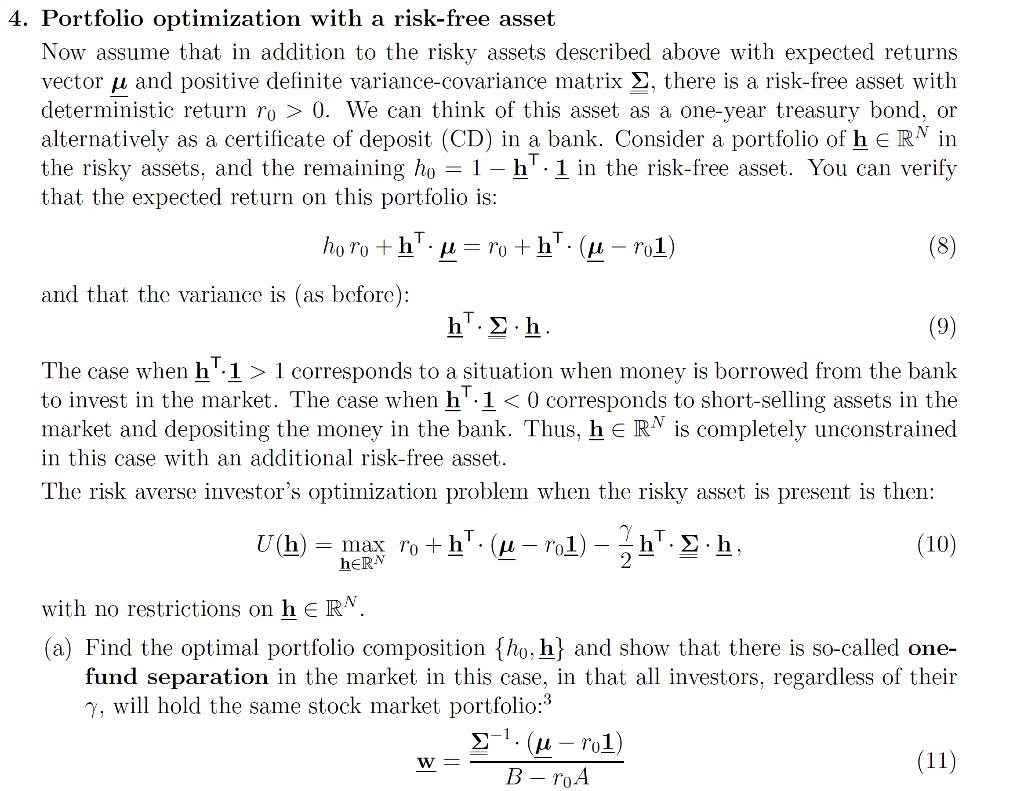
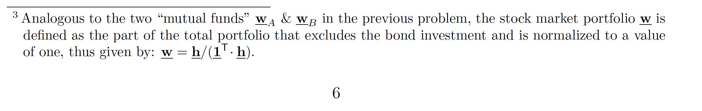
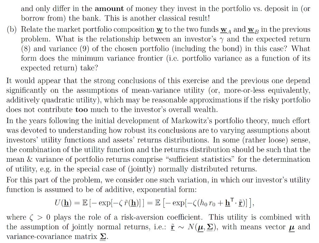
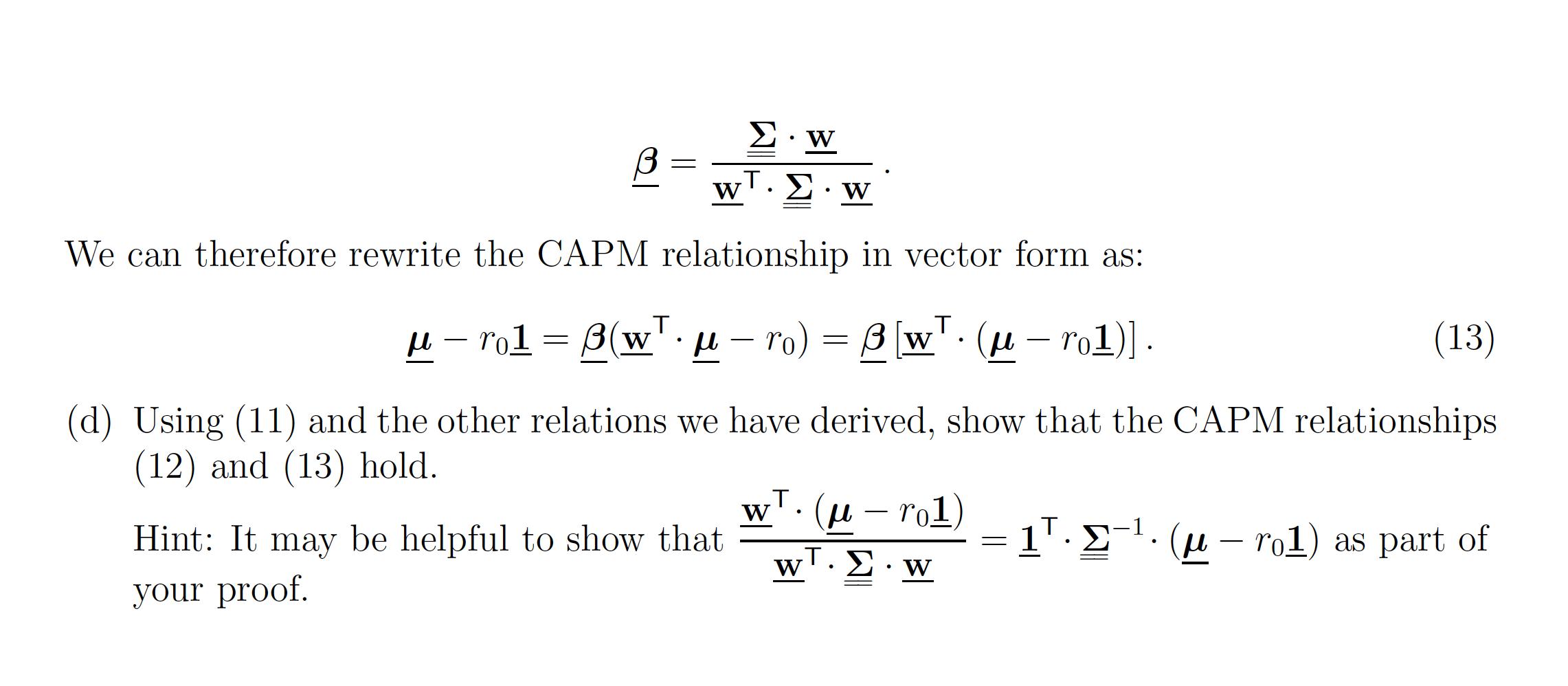
4. Portfolio optimization with a risk-free asset Now assume that in addition to the risky assets described above with expected returns vector and positive definite variance-covariance matrix , there is a risk-free asset with deterministic return ro >0. We can think of this asset as a one-year treasury bond, or alternatively as a certificate of deposit (CD) in a bank. Consider a portfolio of h = RN in the risky assets, and the remaining ho = 1h 1 in the risk-free asset. You can verify that the expected return on this portfolio is: T horo+hro+h. (-rol) and that the variance is (as before): h..h. (8) (9) The case when h1> 1 corresponds to a situation when money is borrowed from the bank to invest in the market. The case when h 1 < 0 corresponds to short-selling assets in the market and depositing the money in the bank. Thus, h = RN is completely unconstrained in this case with an additional risk-free asset. The risk averse investor's optimization problem when the risky asset is present is then: . U (h) = max ro+h (-ro1) -h.h. with no restrictions on h = RN. (10) (a) Find the optimal portfolio composition {ho, h} and show that there is so-called one- fund separation in the market in this case, in that all investors, regardless of their Y, will hold the same stock market portfolio:3 1 W (-rol) B-roA (11) Analogous to the two "mutual funds" WA & WB in the previous problem, the stock market portfolio w is defined as the part of the total portfolio that excludes the bond investment and is normalized to a value of one, thus given by: w=h/(1. h). 6 and only differ in the amount of money they invest in the portfolio vs. deposit in (or borrow from) the bank. This is another classical result! (b) Relate the market portfolio composition w to the two funds WA and WB in the previous problem. What is the relationship between an investor's y and the expected return (8) and variance (9) of the chosen portfolio (including the bond) in this case? What form does the minimum variance frontier (i.e. portfolio variance as a function of its expected return) take? It would appear that the strong conclusions of this exercise and the previous one depend significantly on the assumptions of mean-variance utility (or, more-or-less equivalently, additively quadratic utility), which may be reasonable approximations if the risky portfolio does not contribute too much to the investor's overall wealth. In the years following the initial development of Markowitz's portfolio theory, much effort was devoted to understanding how robust its conclusions are to varying assumptions about investors' utility functions and assets' returns distributions. In some (rather loose) sense, the combination of the utility function and the returns distribution should be such that the mean & variance of portfolio returns comprise "sufficient statistics" for the determination of utility, e.g. in the special case of (jointly) normally distributed returns. For this part of the problem, we consider one such variation, in which our investor's utility function is assumed to be of additive, exponential form: U(h) = E [ exp[ (h)]] = E [ exp[-((horo+h. r)]], where 0 plays the role of a risk-aversion coefficient. This utility is combined with the assumption of jointly normal returns, i.e.: ~ N(, ), with means vector and variance-covariance matrix . (c) Using the mean and variance properties of established thus far and the fact that: E[e] = ekx+k02/2 for a normally distributed variable ~ N(,), show that the portfolio optimization problem can be mapped into the form (10) and relate the coefficient y to . Hint: use the chain rule and consider the first-order optimality conditions for a strictly monotonic R R function of another RN R function, i.e. g(f(x)). The Capital Asset Pricing Model (CAPM) may be the most influential asset pricing model of all time, relating the expected returns of an asset with the extent to which its returns co-vary with the stock market. Specifically, given that the random return of stock n is fn, while the (random) return of the stock market is fmkt, with variance and expected +2 return mkt, the CAPM asserts that: mkt Cov(n, Tmkt) Hn-ro = Bn (mkt - To), where n = mkt (12) In our model with investors with mean-variance preferences, everyone invests in portfolio w given by (11), so w must be the stock market portfolio, leading to mkt . .. =w, and It is then straightforward to show that the vector = (1,..., BN) RN of covariances between stocks and the market, normalized by the market's variance, is given by: 7 .w = W I..w We can therefore rewrite the CAPM relationship in vector form as: T T ro = (w ro) = [w. ( ro1)] . - (w . (13) (d) Using (11) and the other relations we have derived, show that the CAPM relationships (12) and (13) hold. Hint: It may be helpful to show that your proof. W wT. (-rol) T = . ( (ro1) as part of I..w W 4. Portfolio optimization with a risk-free asset Now assume that in addition to the risky assets described above with expected returns vector and positive definite variance-covariance matrix , there is a risk-free asset with deterministic return ro >0. We can think of this asset as a one-year treasury bond, or alternatively as a certificate of deposit (CD) in a bank. Consider a portfolio of h = RN in the risky assets, and the remaining ho = 1h 1 in the risk-free asset. You can verify that the expected return on this portfolio is: T horo+hro+h. (-rol) and that the variance is (as before): h..h. (8) (9) The case when h1> 1 corresponds to a situation when money is borrowed from the bank to invest in the market. The case when h 1 < 0 corresponds to short-selling assets in the market and depositing the money in the bank. Thus, h = RN is completely unconstrained in this case with an additional risk-free asset. The risk averse investor's optimization problem when the risky asset is present is then: . U (h) = max ro+h (-ro1) -h.h. with no restrictions on h = RN. (10) (a) Find the optimal portfolio composition {ho, h} and show that there is so-called one- fund separation in the market in this case, in that all investors, regardless of their Y, will hold the same stock market portfolio:3 1 W (-rol) B-roA (11) Analogous to the two "mutual funds" WA & WB in the previous problem, the stock market portfolio w is defined as the part of the total portfolio that excludes the bond investment and is normalized to a value of one, thus given by: w=h/(1. h). 6 and only differ in the amount of money they invest in the portfolio vs. deposit in (or borrow from) the bank. This is another classical result! (b) Relate the market portfolio composition w to the two funds WA and WB in the previous problem. What is the relationship between an investor's y and the expected return (8) and variance (9) of the chosen portfolio (including the bond) in this case? What form does the minimum variance frontier (i.e. portfolio variance as a function of its expected return) take? It would appear that the strong conclusions of this exercise and the previous one depend significantly on the assumptions of mean-variance utility (or, more-or-less equivalently, additively quadratic utility), which may be reasonable approximations if the risky portfolio does not contribute too much to the investor's overall wealth. In the years following the initial development of Markowitz's portfolio theory, much effort was devoted to understanding how robust its conclusions are to varying assumptions about investors' utility functions and assets' returns distributions. In some (rather loose) sense, the combination of the utility function and the returns distribution should be such that the mean & variance of portfolio returns comprise "sufficient statistics" for the determination of utility, e.g. in the special case of (jointly) normally distributed returns. For this part of the problem, we consider one such variation, in which our investor's utility function is assumed to be of additive, exponential form: U(h) = E [ exp[ (h)]] = E [ exp[-((horo+h. r)]], where 0 plays the role of a risk-aversion coefficient. This utility is combined with the assumption of jointly normal returns, i.e.: ~ N(, ), with means vector and variance-covariance matrix . (c) Using the mean and variance properties of established thus far and the fact that: E[e] = ekx+k02/2 for a normally distributed variable ~ N(,), show that the portfolio optimization problem can be mapped into the form (10) and relate the coefficient y to . Hint: use the chain rule and consider the first-order optimality conditions for a strictly monotonic R R function of another RN R function, i.e. g(f(x)). The Capital Asset Pricing Model (CAPM) may be the most influential asset pricing model of all time, relating the expected returns of an asset with the extent to which its returns co-vary with the stock market. Specifically, given that the random return of stock n is fn, while the (random) return of the stock market is fmkt, with variance and expected +2 return mkt, the CAPM asserts that: mkt Cov(n, Tmkt) Hn-ro = Bn (mkt - To), where n = mkt (12) In our model with investors with mean-variance preferences, everyone invests in portfolio w given by (11), so w must be the stock market portfolio, leading to mkt . .. =w, and It is then straightforward to show that the vector = (1,..., BN) RN of covariances between stocks and the market, normalized by the market's variance, is given by: 7 .w = W I..w We can therefore rewrite the CAPM relationship in vector form as: T T ro = (w ro) = [w. ( ro1)] . - (w . (13) (d) Using (11) and the other relations we have derived, show that the CAPM relationships (12) and (13) hold. Hint: It may be helpful to show that your proof. W wT. (-rol) T = . ( (ro1) as part of I..w W