

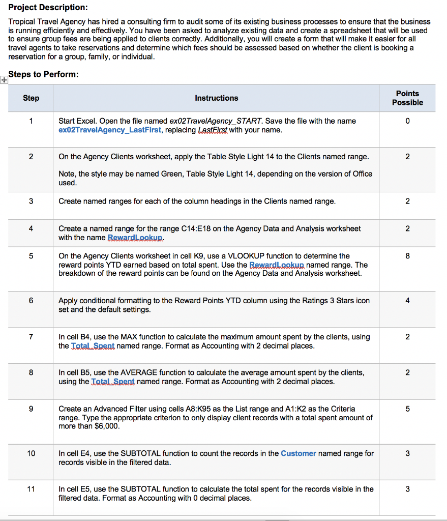
Project Description: Tropical Travel Agency has hired a consulting firm to audit some of its existing...
Fantastic news! We've Found the answer you've been seeking!
Question:
Transcribed Image Text:
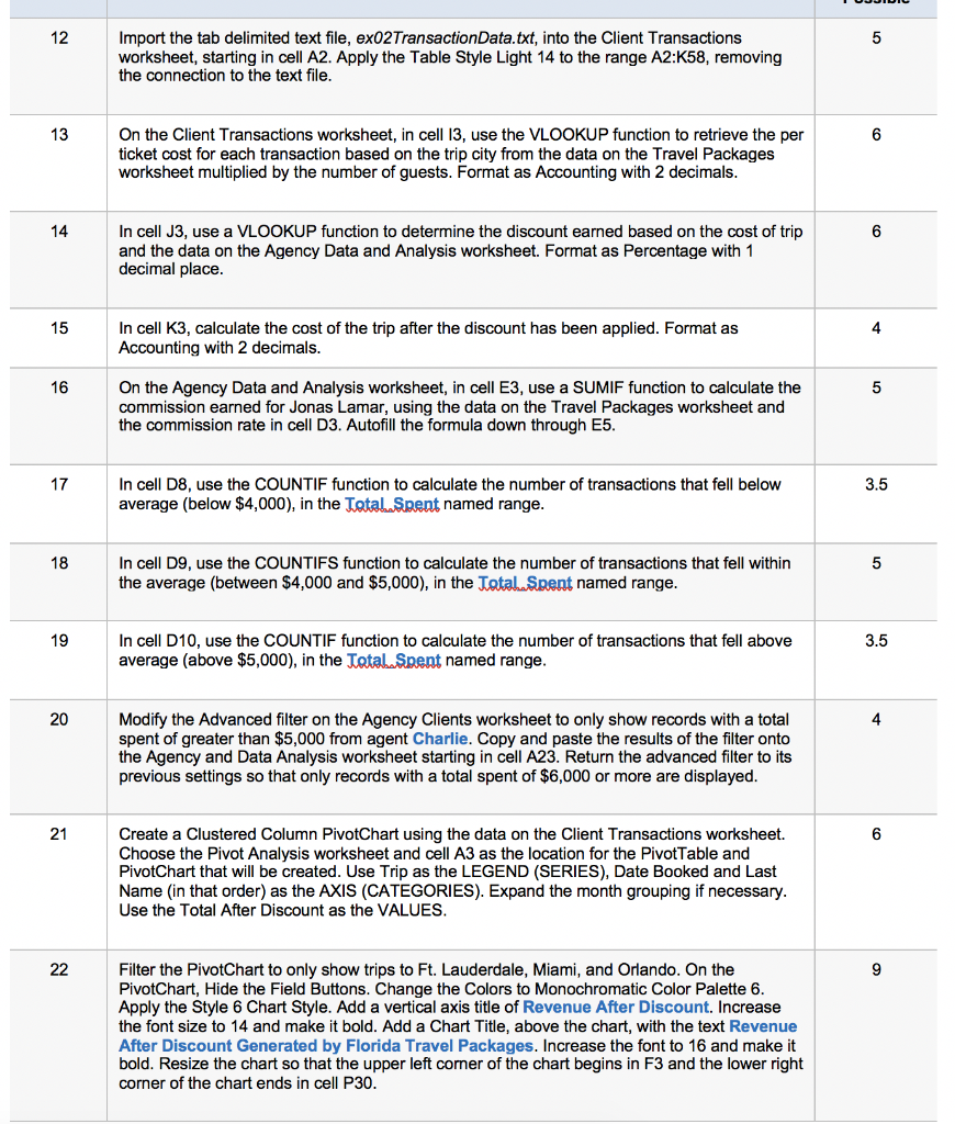
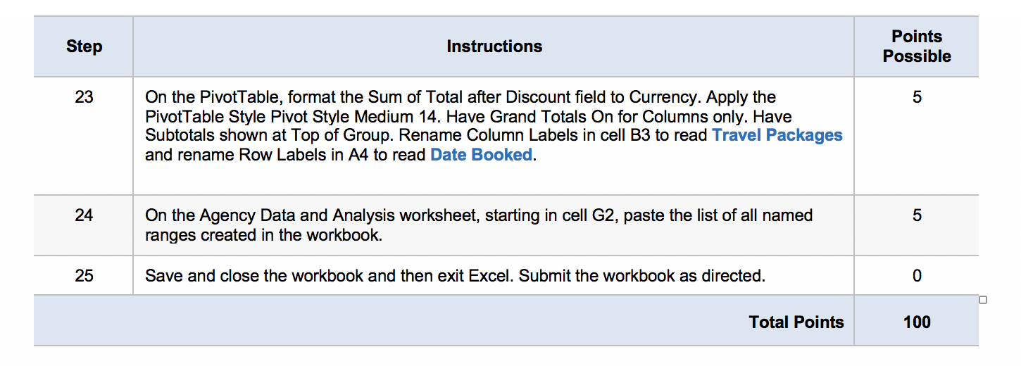
Project Description: Tropical Travel Agency has hired a consulting firm to audit some of its existing business processes to ensure that the business is running efficiently and effectively. You have been asked to analyze existing data and create a spreadsheet that will be used to ensure group fees are being applied to clients correctly. Additionally, you will create a form that will make it easier for all travel agents to take reservations and determine which fees should be assessed based on whether the client is booking a reservation for a group, family, or individual. Steps to Perform: Step 1 2 3 4 5 6 7 8 9 10 11 Instructions Start Excel. Open the file named ex02TravelAgency_START. Save the file with the name ex02TravelAgency_LastFirst, replacing LastFirst with your name. On the Agency Clients worksheet, apply the Table Style Light 14 to the Clients named range. Note, the style may be named Green, Table Style Light 14, depending on the version of Office used. Create named ranges for each of the column headings in the Clients named range. Create a named range for the range C14:E18 on the Agency Data and Analysis worksheet with the name Rewardlookup. On the Agency Clients worksheet in cell K9, use a VLOOKUP function to determine the reward points YTD earned based on total spent. Use the Rewardlookup named range. The breakdown of the reward points can be found on the Agency Data and Analysis worksheet. Apply conditional formatting to the Reward Points YTD column using the Ratings 3 Stars icon set and the default settings. In cell B4, use the MAX function to calculate the maximum amount spent by the clients, using the Total Spent named range. Format as Accounting with 2 decimal places. In cell B5, use the AVERAGE function to calculate the average amount spent by the clients, using the Total Spent named range. Format as Accounting with 2 decimal places. Create an Advanced Filter using cells A8:K95 as the List range and A1:K2 as the Criteria range. Type the appropriate criterion to only display client records with a total spent amount of more than $6,000. In cell E4, use the SUBTOTAL function to count the records in the Customer named range for records visible in the filtered data. In cell E5, use the SUBTOTAL function to calculate the total spent for the records visible in the filtered data. Format as Accounting with 0 decimal places. Points Possible 0 2 2 2 8 4 2 2 5 3 3 12 13 14 15 16 17 18 19 20 21 22 ex02TransactionData.txt, into the Client Transactions Import the tab delimited text file, worksheet, starting in cell A2. Apply the Table Style Light 14 to the range A2:K58, removing the connection to the text file. On the Client Transactions worksheet, in cell 13, use the VLOOKUP function to retrieve the per ticket cost for each transaction based on the trip city from the data on the Travel Packages worksheet multiplied by the number of guests. Format as Accounting with 2 decimals. In cell J3, use a VLOOKUP function to determine the discount earned based on the cost of trip and the data on the Agency Data and Analysis worksheet. Format as Percentage with 1 decimal place. In cell K3, calculate the cost of the trip after the discount has been applied. Format as Accounting with 2 decimals. On the Agency Data and Analysis worksheet, in cell E3, use a SUMIF function to calculate the commission earned for Jonas Lamar, using the data on the Travel Packages worksheet and the commission rate in cell D3. Autofill the formula down through E5. In cell D8, use the COUNTIF function to calculate the number of transactions that fell below average (below $4,000), in the Total Spent named range. In cell D9, use the COUNTIFS function to calculate the number of transactions that fell within the average (between $4,000 and $5,000), in the Total Spent named range. In cell D10, use the COUNTIF function to calculate the number of transactions that fell above average (above $5,000), in the Total Spent named range. Modify the Advanced filter on the Agency Clients worksheet to only show records with a total spent of greater than $5,000 from agent Charlie. Copy and paste the results of the filter onto the Agency and Data Analysis worksheet starting in cell A23. Return the advanced filter to its previous settings so that only records with a total spent of $6,000 or more are displayed. Create a Clustered Column PivotChart using the data on the Client Transactions worksheet. Choose the Pivot Analysis worksheet and cell A3 as the location for the PivotTable and PivotChart that will be created. Use Trip as the LEGEND (SERIES), Date Booked and Last Name (in that order) as the AXIS (CATEGORIES). Expand the month grouping if necessary. Use the Total After Discount as the VALUES. Filter the PivotChart to only show trips to Ft. Lauderdale, Miami, and Orlando. On the PivotChart, Hide the Field Buttons. Change the Colors to Monochromatic Color Palette 6. Apply the Style 6 Chart Style. Add a vertical axis title of Revenue After Discount. Increase the font size to 14 and make it bold. Add a Chart Title, above the chart, with the text Revenue After Discount Generated by Florida Travel Packages. Increase the font to 16 and make it bold. Resize the chart so that the upper left corner of the chart begins in F3 and the lower right corner of the chart ends in cell P30. 5 6 6 4 5 3.5 5 3.5 4 6 9 Step 23 24 25 Instructions On the PivotTable, format the Sum of Total after Discount field to Currency. Apply the PivotTable Style Pivot Style Medium 14. Have Grand Totals On for Columns only. Have Subtotals shown at Top of Group. Rename Column Labels in cell B3 to read Travel Packages and rename Row Labels in A4 to read Date Booked. On the Agency Data and Analysis worksheet, starting in cell G2, paste the list of all named ranges created in the workbook. Save and close the workbook and then exit Excel. Submit the workbook as directed. Total Points Points Possible 5 5 0 100 Project Description: Tropical Travel Agency has hired a consulting firm to audit some of its existing business processes to ensure that the business is running efficiently and effectively. You have been asked to analyze existing data and create a spreadsheet that will be used to ensure group fees are being applied to clients correctly. Additionally, you will create a form that will make it easier for all travel agents to take reservations and determine which fees should be assessed based on whether the client is booking a reservation for a group, family, or individual. Steps to Perform: Step 1 2 3 4 5 6 7 8 9 10 11 Instructions Start Excel. Open the file named ex02TravelAgency_START. Save the file with the name ex02TravelAgency_LastFirst, replacing LastFirst with your name. On the Agency Clients worksheet, apply the Table Style Light 14 to the Clients named range. Note, the style may be named Green, Table Style Light 14, depending on the version of Office used. Create named ranges for each of the column headings in the Clients named range. Create a named range for the range C14:E18 on the Agency Data and Analysis worksheet with the name Rewardlookup. On the Agency Clients worksheet in cell K9, use a VLOOKUP function to determine the reward points YTD earned based on total spent. Use the Rewardlookup named range. The breakdown of the reward points can be found on the Agency Data and Analysis worksheet. Apply conditional formatting to the Reward Points YTD column using the Ratings 3 Stars icon set and the default settings. In cell B4, use the MAX function to calculate the maximum amount spent by the clients, using the Total Spent named range. Format as Accounting with 2 decimal places. In cell B5, use the AVERAGE function to calculate the average amount spent by the clients, using the Total Spent named range. Format as Accounting with 2 decimal places. Create an Advanced Filter using cells A8:K95 as the List range and A1:K2 as the Criteria range. Type the appropriate criterion to only display client records with a total spent amount of more than $6,000. In cell E4, use the SUBTOTAL function to count the records in the Customer named range for records visible in the filtered data. In cell E5, use the SUBTOTAL function to calculate the total spent for the records visible in the filtered data. Format as Accounting with 0 decimal places. Points Possible 0 2 2 2 8 4 2 2 5 3 3 12 13 14 15 16 17 18 19 20 21 22 ex02TransactionData.txt, into the Client Transactions Import the tab delimited text file, worksheet, starting in cell A2. Apply the Table Style Light 14 to the range A2:K58, removing the connection to the text file. On the Client Transactions worksheet, in cell 13, use the VLOOKUP function to retrieve the per ticket cost for each transaction based on the trip city from the data on the Travel Packages worksheet multiplied by the number of guests. Format as Accounting with 2 decimals. In cell J3, use a VLOOKUP function to determine the discount earned based on the cost of trip and the data on the Agency Data and Analysis worksheet. Format as Percentage with 1 decimal place. In cell K3, calculate the cost of the trip after the discount has been applied. Format as Accounting with 2 decimals. On the Agency Data and Analysis worksheet, in cell E3, use a SUMIF function to calculate the commission earned for Jonas Lamar, using the data on the Travel Packages worksheet and the commission rate in cell D3. Autofill the formula down through E5. In cell D8, use the COUNTIF function to calculate the number of transactions that fell below average (below $4,000), in the Total Spent named range. In cell D9, use the COUNTIFS function to calculate the number of transactions that fell within the average (between $4,000 and $5,000), in the Total Spent named range. In cell D10, use the COUNTIF function to calculate the number of transactions that fell above average (above $5,000), in the Total Spent named range. Modify the Advanced filter on the Agency Clients worksheet to only show records with a total spent of greater than $5,000 from agent Charlie. Copy and paste the results of the filter onto the Agency and Data Analysis worksheet starting in cell A23. Return the advanced filter to its previous settings so that only records with a total spent of $6,000 or more are displayed. Create a Clustered Column PivotChart using the data on the Client Transactions worksheet. Choose the Pivot Analysis worksheet and cell A3 as the location for the PivotTable and PivotChart that will be created. Use Trip as the LEGEND (SERIES), Date Booked and Last Name (in that order) as the AXIS (CATEGORIES). Expand the month grouping if necessary. Use the Total After Discount as the VALUES. Filter the PivotChart to only show trips to Ft. Lauderdale, Miami, and Orlando. On the PivotChart, Hide the Field Buttons. Change the Colors to Monochromatic Color Palette 6. Apply the Style 6 Chart Style. Add a vertical axis title of Revenue After Discount. Increase the font size to 14 and make it bold. Add a Chart Title, above the chart, with the text Revenue After Discount Generated by Florida Travel Packages. Increase the font to 16 and make it bold. Resize the chart so that the upper left corner of the chart begins in F3 and the lower right corner of the chart ends in cell P30. 5 6 6 4 5 3.5 5 3.5 4 6 9 Step 23 24 25 Instructions On the PivotTable, format the Sum of Total after Discount field to Currency. Apply the PivotTable Style Pivot Style Medium 14. Have Grand Totals On for Columns only. Have Subtotals shown at Top of Group. Rename Column Labels in cell B3 to read Travel Packages and rename Row Labels in A4 to read Date Booked. On the Agency Data and Analysis worksheet, starting in cell G2, paste the list of all named ranges created in the workbook. Save and close the workbook and then exit Excel. Submit the workbook as directed. Total Points Points Possible 5 5 0 100
Expert Answer:

Related Book For 
Business Statistics A Decision Making Approach
ISBN: 9780133021844
9th Edition
Authors: David F. Groebner, Patrick W. Shannon, Phillip C. Fry
Posted Date:
Students also viewed these accounting questions
-
3 4 5 6 7 8 9 10 11 12 13 A 14 Cost of the Asset 15 Life of the Asset in Years 16 Book Value of the Asset after 5 years 17 Depreciable Basis 18 Yearly depreciation 19 After tax Salvage Value in year...
-
You have been asked to determine if two different production processes have different mean numbers of units produced per hour. Process 1 has a mean defined as 1 and process 2 has a mean defined as 2....
-
You have been asked to determine if two different production processes have different mean numbers of units produced per hour. Process 1 has a mean defined as m1 and process 2 has a mean defined as...
-
ed The Engine Guys produces specialized engines for "snow climber buses. The company's normal monthly production volume is 2,500 engines, whereas its monthly production capacity is 5,000 engines. The...
-
Dr. Lucy Zang, a noted local podiatrist, plans to open a retail shoe store specializing in hard- to- find footwear for people with feet problems such as bunions, flat feet, mallet toes, diabetic...
-
Rosatos supervisor questions her assumption that Taiwan Semiconductor will have no premium at the end of her forecast period. Rosato assesses the effect of a terminal value based on a perpetuity of...
-
Teddys daily budget constraint is shown in the following chart. Teddys employer pays him a base wage rate plus overtime if he works more than the standard hours. What is Teddys daily nonlabor income?...
-
The following are misstatements that might be found in the client's year-end cash balance (assume that the balance sheet date is June 30): 1. The outstanding checks on the June 30 bank reconciliation...
-
Question 17 (1 point) If the credit to record the payment of an account payable is not posted Liabilities will be understated Expenses will be understated Cash will be overstated Which statement is...
-
The following data relate to the operations of Shilow Company, a wholesale distributor of consumer goods: Current assets as of March 31: Cash $ 8,000 Accounts receivable 20,000 Inventory 36,000...
-
Explain the advantages of maturity of industries as well as the possible limitations.
-
Assume that Freezeqwik Ltd (Activity 10.16) wishes to reduce its OCC by 30 days. Evaluate each of the options available to this business.
-
The following figures relate to the retail business of Daisy King for the month of July. Goods sold fall into two categories, X and Y. You are to calculate for each category of goods: (a) Cost of...
-
Styrene can be hydrogenated to ethyl benzene at moderate conditions in both the liquid and the gas phases. Calculate the equilibrium compositions in the vapor and liquid phases of hydrogen, styrene,...
-
A home heating system maintains the indoor temperature at 20 C. The outside temperature is 0 C. A furnace burns natural gas to heat a 1:4 mixture of outside and inside air. The resulting air is at a...
-
Yaso is in business buying and selling goods on credit. He is concerned that although his business is making a good profit, his balance at the bank is not increasing. The following information is...
-
Suppose that the current spot exchange rate is S=1.26$/. You observe the following American style options: a. An American put on the Euro with K=1.30$/, 3 months till expiration that is selling in...
-
Write a declaration for each of the following: a. A line that extends from point (60, 100) to point (30, 90) b. A rectangle that is 20 pixels wide, 100 pixels high, and has its upper-left corner at...
-
The Miltmore Corporation performs consulting services for companies that think they have image problems. Recently, the Bluedot Beer Company approached Miltmore. Bluedot executives were concerned that...
-
Discuss any advantages a graph showing a whole set of data has over a single measure, such as an average.
-
Suppose a random sample of 137 households in Detroit was selected to determine the average annual household spending on food at home for Detroit residents. The sample results are contained in the...
-
The following accounts and amounts (balances are normal balances) were taken from the records of Prider Manufacturers Ltd at 30 June 2019. Required (a) Prepare a cost of goods manufactured statement...
-
The following data were taken from the records of Manik Manufacturing Ltd for the year ended 30 June 2019. Required (a) Prepare the cost of goods manufactured schedule for the year ended 30 June...
-
The following demonstration problem illustrates the use of the general journal, the four special journals introduced here, and the general ledger with two subsidiary ledgers. Sidney Carton began...

Study smarter with the SolutionInn App