Provide unit tests to prove that this implementation is correcct for the Black Scholes code below. Also write a README.md file for the same :

import numpy as np import pandas as pd import matplotlib.pyplot as plt from mpl_toolkits.mplot3d import Axes3D

class BSMPDESolver: def __init__(self, N, M, vol, int_rate, option_type, strike, expiration): self.N = N self.M = M self.vol = vol self.int_rate = int_rate self.option_type = option_type self.strike = strike self.expiration = expiration

def solve_pde(self): S = np.linspace(0, 3 * self.strike, self.N + 1) # Asset array dS = 3 * self.strike / self.N # 'Infinity' is twice the strike dt = 0.9 / self.vol ** 2 / self.N ** 2 # For stability V = np.zeros((self.N + 1, self.M + 1)) # Option value array q = 1 if self.option_type == "call" else -1

# Payoff function V[:, 0] = np.maximum(q * (S - self.strike), 0)

for k in range(1, self.M + 1): # Time loop NTS = int(self.expiration / dt) + 1 # Recalculate NTS based on time step dt = self.expiration / NTS # To ensure that expiration is an integer number of time steps away

# Central difference delta = (V[2:, k - 1] - V[:-2, k - 1]) / (2 * dS) gamma = (V[2:, k - 1] - 2 * V[1:-1, k - 1] + V[:-2, k - 1]) / dS**2

# Black-Scholes equation theta = -0.5 * self.vol ** 2 * S[1:-1] ** 2 * gamma - \ self.int_rate * S[1:-1] * delta + self.int_rate * V[1:-1, k - 1]

# Update option value V[1:-1, k] = V[1:-1, k - 1] - dt * theta

# Boundary conditions V[0, k] = V[0, k - 1] * (1 - self.int_rate * dt) # at S=0 V[-1, k] = 2 * V[-2, k] - V[-3, k] # at S=infinity

asset_range = np.linspace(0, 3 * self.strike, self.N + 1) # Asset price range time_steps = np.linspace(0, self.expiration, self.M + 1) rounded_time_steps = np.round(time_steps, decimals=3) df = pd.DataFrame(V, index=asset_range, columns=rounded_time_steps).round(3)

return df

def build_coefficient_matrix(self): # Implement the method to build the coefficient matrix if needed pass

def build_rhs_vector(self): # Implement the method to build the right-hand side vector if needed pass

from pde1 import BSMPDESolver # Example usage N = 100 M = 100 sigma = 0.2 r = 0.05 K = 30 T = 2

solver = BSMPDESolver(N, M, sigma, r, "call", K, T) option_df = solver.solve_pde()

# Plotting fig = plt.figure(figsize=(10, 10)) ax = fig.add_subplot(111, projection='3d')

X, Y = np.meshgrid(option_df.columns, option_df.index) Z = option_df.values

surf = ax.plot_surface(X, Y, Z, cmap='coolwarm')

ax.set_xlabel('Time') ax.set_ylabel('Stock Price') ax.set_zlabel('Option Price') ax.set_title('Option Value Surface Plot')

fig.colorbar(surf, shrink=0.5, aspect=5) plt.show()

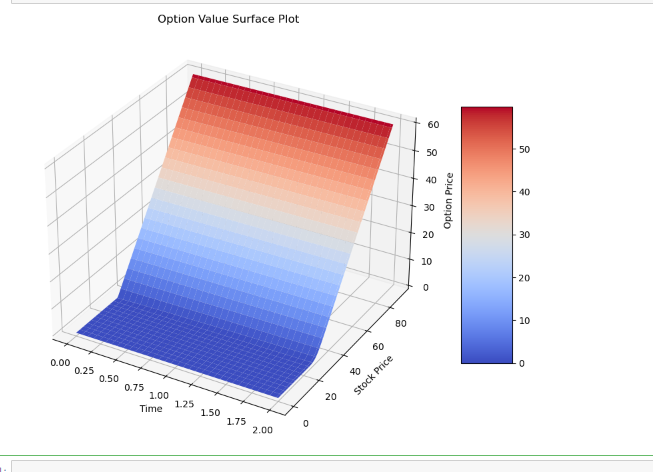
Option Value Surface Plot