[PYTHON] In this problem we'll figure out how to fit linear SVM models to data using sklearn. Consider the data shown below.

import numpy as np from sklearn.datasets import make_blobs from matplotlib.colors import Normalize import matplotlib.pyplot as plt %matplotlib inline

def linear_plot(X, y, w=None, b=None): mycolors = {"blue": "steelblue", "red": "#a76c6e", "green": "#6a9373"} colors = [mycolors["red"] if yi==1 else mycolors["blue"] for yi in y] # Plot data fig, ax = plt.subplots(nrows=1, ncols=1, figsize=(8,8)) ax.scatter(X[:,0], X[:,1], color=colors, s=150, alpha=0.95, zorder=2) # Plot boundaries lower_left = np.min([np.min(X[:,0]), np.min(X[:,1])]) upper_right = np.max([np.max(X[:,0]), np.max(X[:,1])]) gap = .1*(upper_right-lower_left) xplot = np.linspace(lower_left-gap, upper_right+gap, 20) if w is not None and b is not None: ax.plot(xplot, (-b - w[0]*xplot)/w[1], color="gray", lw=2, zorder=1) ax.plot(xplot, ( 1 -b - w[0]*xplot)/w[1], color="gray", lw=2, ls="--", zorder=1) ax.plot(xplot, (-1 -b - w[0]*xplot)/w[1], color="gray", lw=2, ls="--", zorder=1) ax.set_xlim([lower_left-gap, upper_right+gap]) ax.set_ylim([lower_left-gap, upper_right+gap]) ax.grid(alpha=0.25)

def part2data(): np.random.seed(1239) X = np.zeros((22,2)) X[0:10,0] = 1.5*np.random.rand(10) X[0:10,1] = 1.5*np.random.rand(10) X[10:20,0] = 1.5*np.random.rand(10) + 1.75 X[10:20,1] = 1.5*np.random.rand(10) + 1 X[20,0] = 1.5 X[20,1] = 2.25 X[21,0] = 1.6 X[21,1] = 0.25 y = np.ones(22) y[10:20] = -1 y[20] = 1 y[21] = -1 return X, y

------------------------------

X, y = part2data() linear_plot(X, y)

TO DO 1: Complete de code below following the previous instructions. Do not change de code, just complete it.

from sklearn.svm import LinearSVC

# TODO: Build a LinearSVC model called lsvm. Train the model and get the parameters, pay attention to the loss parameter lsvm = None # complete your code here

# use this code to plot the resulting model w = lsvm.coef_[0] b = lsvm.intercept_ print(w,b) linear_plot(X, y, w=w, b=b)

TO DO 2: Experiment with different values of C. Answer the following question in your Peer Review for the week: How does the choice of C affect the nature of the decision boundary and the associated margin?

from sklearn.svm import LinearSVC

# TODO: Change the svm model parameter and plot the result.

# complete your code here

TO DO 3: Set C=3 and compare the results you get when using the hinge vs the squared_hinge values for the loss parameter. Explain your observations. Compare hinge loss vs. squared hinge loss.

TO DO 4: In general, how does the choice of C affect the bias and variance of the model?

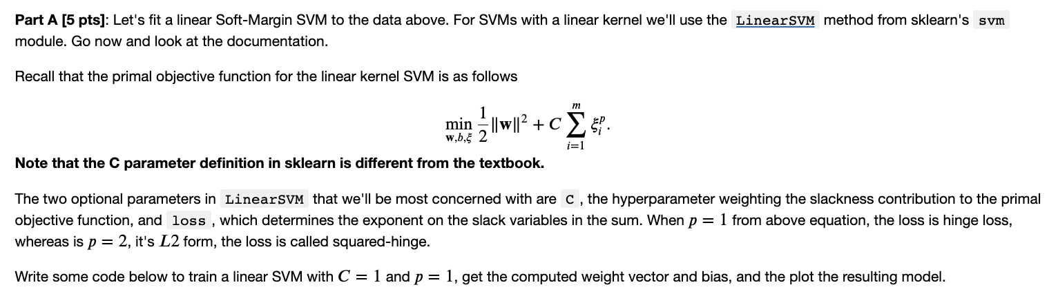
Part A [5 pts]: Let's fit a linear Soft-Margin SVM to the data above. For SVMs with a linear kernel we'll use the method from sklearn's module. Go now and look at the documentation. Recall that the primal objective function for the linear kernel SVM is as follows minw,b,21w2+Ci=1mip. Note that the C parameter definition in sklearn is different from the textbook. The two optional parameters in that we'll be most concerned with are C, the hyperparameter weighting the slackness contribution to the primal objective function, and loss, which determines the exponent on the slack variables in the sum. When p=1 from above equation, the loss is hinge loss, whereas is p=2, it's L2 form, the loss is called squared-hinge. Write some code below to train a linear SVM with C=1 and p=1, get the computed weight vector and bias, and the plot the resulting model