Question:

While reading the case, look for inputs to the model that are subject to uncertainty. This means any input to the model that is not fixed and could change. The case provides context that should help you find these inputs through the reading. Hint: there are at least 6 inputs. What are the 6 inputs and why?

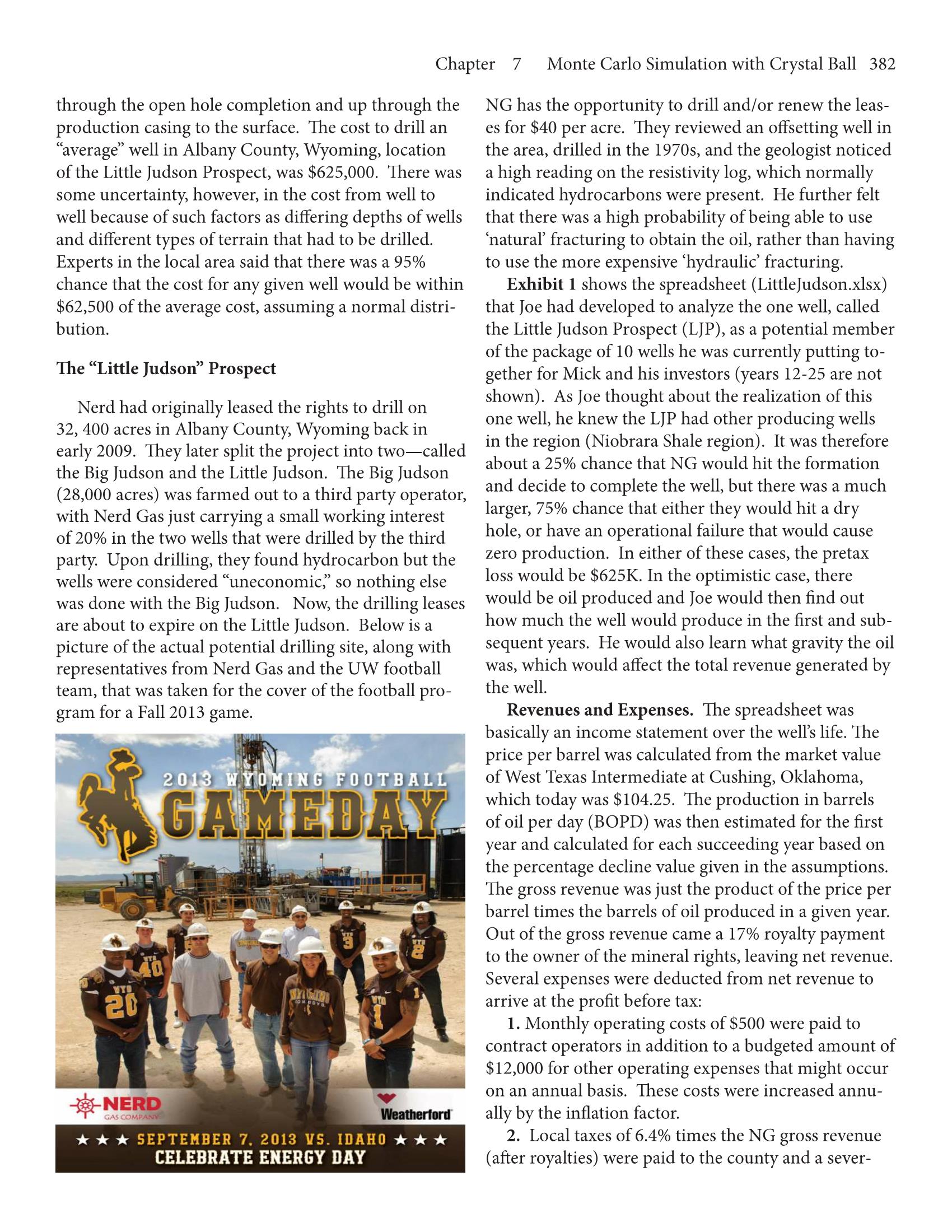
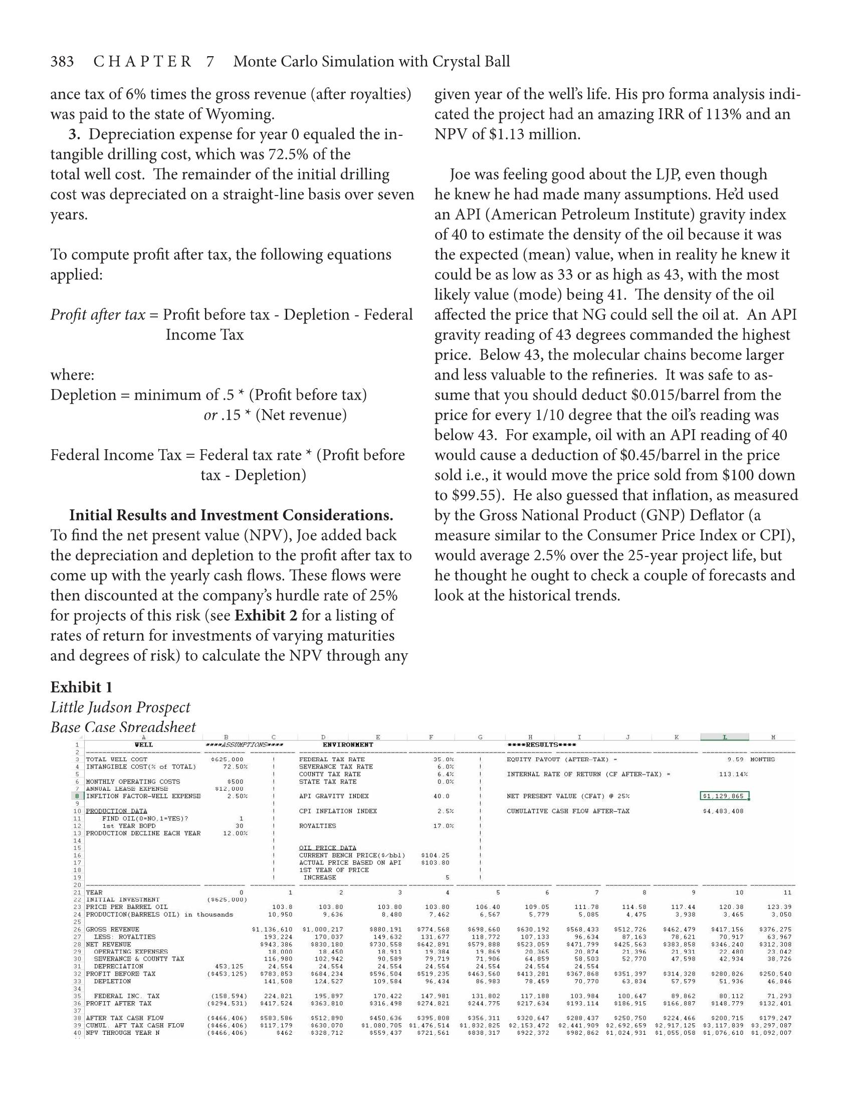
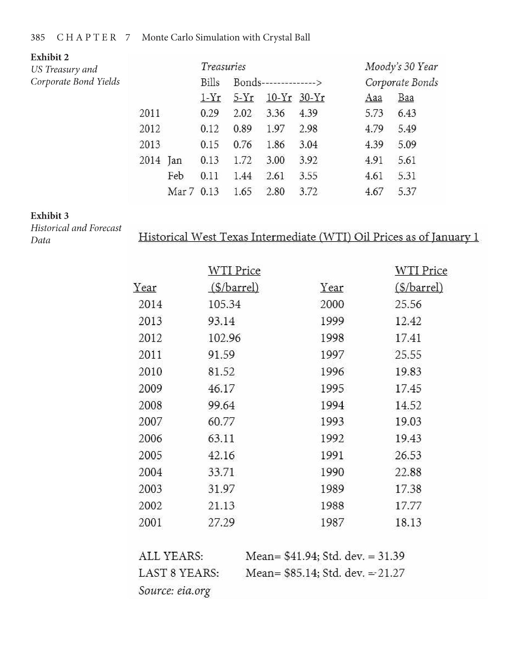
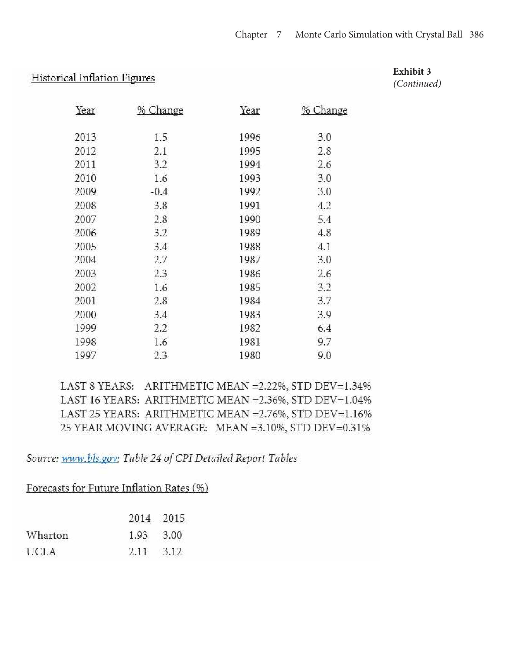
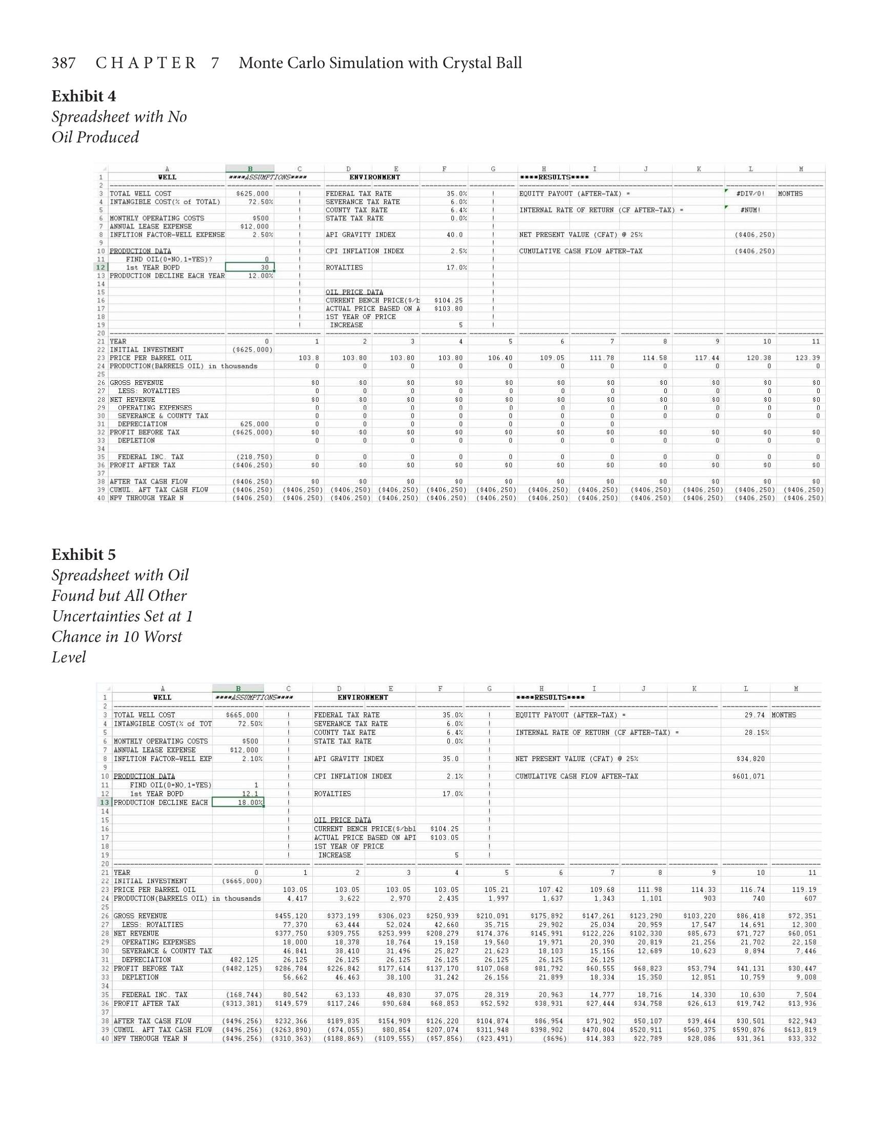
Chapter Monte Carlo Simulation with Crystal Ball 380 Case Study 3 : Little Judson Prospect October 15 was another beautiful , blue sky day in Bureau and was the state of Wyoming's first - ev sfirst - ever western Albany County , Wyoming . Mick McMy recipient of the awar could see some cattle grazing the fields on the high In 2008 , Nerd Gas Company contracted with the plains dessert out in front of him . He was grateful for Idaho National Laboratory ( INL ) to conduct a feasibil the bucolic setting and his generous circumstances ity study investigating the technical and economic via which were made possible by his doing very well wi the bility of locating a natural gas - to -liquids ( GIL ) facility some of his investments , one of which now required in the state of Wyoming Initial feedback delivered by some concentration . Mick was the founder and Presi IN suggested Nerd continue to advance the project dent of Nerd Gas Company . The decision at hand was Nerd has been working with technology providers and whether to drill an oil well known internally as the internally as the Lit the state of Wyoming in a proposed modular - designed the Judson Prospect or not in his effort to try to chase GIL project located in central Wyoming . the Niobrara shale oil play In 2011 , Nerd Gas , along with three local partners possessing significant geologic and exploration exper The Company tise , formed Stakeholder Energy , LLC . Stakeholder was formed to pursue large - scale uranium exploration Founded by Mick MCMurry in 1996 , Nerd Gas in Converse County , Wyoming . Stakeholder has leased Company , LLC is a private , Wyoming - based energy significant acreage ideally positioned between a urani investment company whose primary focus is on the um processing facility and the uranium mine sites efficient and responsible exploration of hydrocarbons The list of Nerd Gas affiliated companies included in Wyoming and the northern Rocky Mountain re High Country Fabrication , Jonah Bank , MSN Field gion Nerd Gas Company is one of Wyoming's leading Services , Nerd Technology and Stakeholder Energy entrepreneurs in energy projects in a state recognized In 2013 , McMurry - related companies employed over for the depth and breadth of its extensive mineral 225 people . resources Another extension of these companies was the very Nerd is currently involved in conventional oil and generous MCMurry foundation , which has given ou gas exploration projects in the Wyoming - Utah Over $49 million dollars to charitable causes in the State of thrust Belt and the Rocky Mountain region . Zones Wyoming since it started in 1998 . Among the many of interest are primarily traditional oil or gas - bearing beneficiaries of their kindness is the University of Cretaceous sand reservoirs , traditi ditional carbonate Wyoming ( UW ) . The foundation had given millions reservoirs voirs and both structural and stratigraphic traps of dollars each to the Wyoming Technology Business Nerd is also currently invested in other potential Incubator , the Jonah field at War Memorial Stadium , energy - producing projects in Wyoming , including the College of Business , and most recently the new pure play " uranium explorati ateway Center on project in the Powder Gateway Cen River Basin Nerd Gas Company is proud of its talented group NERD's Entry into Oil & Natural Gas of professionals on staff that have spent the majority of their careers focusing on Rocky Mountain reservoirs At the time of its founding Nerd Gas Company was and solving energy production challenges Profession a successful working interest partner in the discovery al expertise includes land management , drilling and and nine - year development of both the prolific ) extraction , completions and production , and in - house nah and Pinedale Anticline Fields in Sublette County energy financial analysis . The combination of strong Wyoming . These fields presented geological challenges capital , seasoned professionals and the owner's entre which required new drilling and hydraulic fracturing preneurial spirit allows Nerd Gas to take advantage of technology in order to successfully extract natural rapidly developing opportunities . In 2007 , Nerd Gas gas in these areas . Jonah Field , which was one of the Company was awarded the Torch Award for B for Business largest on - shore natural gas discoveries in the USA Ethics by the Rocky Mountain tain Region Better Business in the early 1990s with 105 trillion cubic feet of gas381 was sold to Alberta Energy {later changed its name to EnCana) in June 2000, and the Anticline Field was sold in November 2001 to Shell Oil. Mick had wanted the company to nd some invest ment opportunities and became convinced that the company could enjoy higher potential returns (30-40% after tax) from natural resource exploration than from other investment opportunities, including real estate, which were yielding 8 10%. Although natural resource exploration was clearly riskier, Mick felt the risk could be lessened by drilling only sites that were part of existing natural resource plays, like the Bakken shale in North Dakota and the Niobrara shale in southeastern Wyoming. Nerd Gas (NG) had drilled four wells recently. It had not been difcult operationally to drill the four wells, but it had been challenging to nd enough highquality investment opportunities. Mick consid- ered wells to be \"good\" if they met all the following criteria: (1) payback of initial cash investment in 36 months or less, (2) at least 25% internal rate of return (IRR) on an after-tax basis, and (3) a positive Net Present Value (NPV). In the rst ve months of production, one of the Wells had already paid back 52% of its initial invest~ ment--well ahead of its target 36-month payout. The other wells were also doing well, and most of them were at least on schedule for meeting their targeted return on investment. Even though things had gone favorably for Mick so far, he knew the pressure was still on him to make good decisions because NG was planning to drill four more in the coming year. Investment Strategy NG acted as the operating partner in the oil and gas drilling ventures it formed, which gave it full respon- sibility for choosing sites and managing the well if oil were found. NG gathered information from the states of Wyoming, Utah and Colorado and from other companies drilling in the vicinity of a well (if they were willing to engage in \"information trading\"). Mick would then put together a lease package for drilling 10, up to 50 wells that he considered good investments based on all the information he had gathered. The total initial investment for a typical package would be around $6 million up to $30 million. NG would retain about 25% ownership and sell the rest to several other working interest partners. As project operator, NC was responsible for hiring C H A P T E R 7 Monte Carlo Simulation with Crystal Ball a general contractor who would actually hire a rm to do the drilling, and NG's engineer Joe Nicholas, who also had an MBA degree from U'N, would determine whether there really was enough oil to make it Worth completing a well. If the decision was to go ahead, the operator would also be in charge of the day-to-day op- erations of a well. NG had entered into a joint venture with Allen and Crouch Petroleum (A&C) of Casper, Wyoming, in which they agreed that A&C would act as the general contractor for all the wells on which NG acted as managing general partner. The rst-year production level varied signicantly from well to well. Joe found the uncertainty could be described with a lognormal probability distribution with a mean of 30 barrels of oil per day (BOPD), a standard deviation of 14 BOPD and a minimum value of zero, of course. Drilling and Developing a Well The most common drilling rig in operation was the rotary rig composed of ve major components-the drill string and bit, the uid-circulating system, the hoisting system, the power plant, and the blowoutpre vention system. To facilitate the drilling process, generally a uid known as drilling mud (composed of water and special chemicals) was circulated around the hole being drilled. In some cases, such as the Little Iudson, air was used as the \"drilling mud.\" The major purpose of the drilling mud was to lubricate the drill bit and to carry to the surface the cuttings that could otherwise remain in the hole and clog it. In the case of the Little Iudson, the drilling proce- dure was divided into 3 stages. The rst 300 feet of hole was drilled with a 121/4\" bit, before running 8-5/8\" diameter metal pipe, referred to as casing into the wellbore. The casing was then cemented in place, stabilizing the rst section of the hole. The second stage of the well was similar to the rst, except a 77/8\" drill bit was used to drill down to 2700 feet, before running another casing string (production casing) into the hole. After cementing the production casing in place NG would be ready to test the well. Because NG was worried about the drilling uids causing forma tion damage, they planned to drill into the productive Niobrara formation using air. If the Well was found to be productive, the producing zone would be left as an 'open hole completion' without any casing supporting the productive zone. This would allow oil to flow Chapter 7 through the open hole completion and up through the production casing to the surface. The cost to drill an \"average\" well in Albany County, Wyoming, location of the Little Judson Prospect, was $625,000. There was some uncertainty, however, in the cost from well to well because of such factors as differing depths of wells and different types of terrain that had to be drilled. Experts in the local area said that there was a 95% chance that the cost for any given well would be within $62,500 of the average cost, assuming a normal distri- bution. The \"Little Judson\" Prospect Nerd had originally leased the rights to drill on 32, 400 acres in Albany County, Wyoming back in early 2009. They later split the project into twocalled the Big Judson and the Little Judson. The Big Judson (28,000 acres) was farmed out to a third party operator, with Nerd Gas just carrying a small working interest of 20% in the two wells that were drilled by the third party. Upon drilling, they found hydrocarbon but the wells were considered \"uneconomic,\" so nothing else was done with the Big Judson. Now, the drilling leases are about to expire on the Little Judson. Below is a picture of the actual potential drilling site, along With representatives from Nerd Gas and the UW football team, that was taken for the cover of the football pro gram for a Fall 2013 game. v If\" I '7 "\"13 DDTBALI. CELEBRATE ENERGY DAY Monte Carlo Simulation with Crystal Ball 382 NG has the opportunity to drill and/or renew the leas es for $40 per acre. They reviewed an offsetting well in the area, drilled in the 19705, and the geologist noticed a high reading on the resistivity log, which normally indicated hydrocarbons were present. He further felt that there was a high probability of being able to use 'natural' fracturing to obtain the oil, rather than having to use the more expensive 'hydraulic' fracturing. Exhibit 1 shows the spreadsheet (LittleJudson.xlsx) that Joe had developed to analyze the one well, called the Little Judson Prospect (LJP), as a potential member of the package of 10 wells he was currently putting to gether for Mick and his investors (years 12-25 are not shown). As Joe thought about the realization of this one well, he knew the LJP had other producing wells in the region (Niobrara Shale region). It was therefore about a 25% chance that NG would hit the formation and decide to complete the well, but there was a much larger, 75% chance that either they would hit a dry hole, or have an operational failure that would cause zero production. In either of these cases, the pretax loss would be $625K. In the optimistic case, there would be oil produced and Joe would then nd out how much the well would produce in the rst and sub- sequent years. He would also learn what gravity the oil was, which would affect the total revenue generated by the well. Revenues and Expenses. The spreadsheet was basically an income statement over the well's life. The price per barrel was calculated from the market value of West Texas Intermediate at Cushing, Oklahoma, which today was $104.25. The production in barrels of oil per day (BOPD) was then estimated for the rst year and calculated for each succeeding year based on the percentage decline value given in the assumptions. The gross revenue was just the product of the price per barrel times the barrels of oil produced in a given year. Out of the gross revenue came a 17% royalty payment to the owner of the mineral rights, leaving net revenue. Several expenses were deducted from net revenue to arrive at the prot before tax: 1. Monthly operating costs of $500 were paid to contract operators in addition to a budgeted amount of $12,000 for other operating expenses that might occur on an annual basis. These costs were increased annu- ally by the ination factor. 2. Local taxes of 6.4% times the NG gross revenue (after royalties) were paid to the county and a sever 383 CHAPTER 7 Monte Carlo Simulation with Crystal Ball ance tax of 6% times the gross revenue (after royalties) given year of the well's life. His pro forma analysis indi- was paid to the state of Wyoming. cated the project had an amazing IRR of 113% and an 3. Depreciation expense for year 0 equaled the in- NPV of $1.13 million. tangible drilling cost, which was 72.5% of the total well cost. The remainder of the initial drilling Joe was feeling good about the LJP, even though cost was depreciated on a straight-line basis over seven he knew he had made many assumptions. He'd used years. an API (American Petroleum Institute) gravity index of 40 to estimate the density of the oil because it was To compute profit after tax, the following equations the expected (mean) value, when in reality he knew it applied: could be as low as 33 or as high as 43, with the most likely value (mode) being 41. The density of the oil Profit after tax = Profit before tax - Depletion - Federal affected the price that NG could sell the oil at. An API Income Tax gravity reading of 43 degrees commanded the highest price. Below 43, the molecular chains become larger where: and less valuable to the refineries. It was safe to as- Depletion = minimum of .5 * (Profit before tax) sume that you should deduct $0.015/barrel from the or .15 * (Net revenue) price for every 1/10 degree that the oil's reading was below 43. For example, oil with an API reading of 40 Federal Income Tax = Federal tax rate * (Profit before would cause a deduction of $0.45/barrel in the price tax - Depletion) sold i.e., it would move the price sold from $100 down to $99.55). He also guessed that inflation, as measured Initial Results and Investment Considerations. by the Gross National Product (GNP) Deflator (a To find the net present value (NPV), Joe added back measure similar to the Consumer Price Index or CPI), the depreciation and depletion to the profit after tax to would average 2.5% over the 25-year project life, but come up with the yearly cash flows. These flows were he thought he ought to check a couple of forecasts and then discounted at the company's hurdle rate of 25% look at the historical trends. for projects of this risk (see Exhibit 2 for a listing of rates of return for investments of varying maturities and degrees of risk) to calculate the NPV through any Exhibit 1 Little Judson Prospect Base Case Spreadsheet WELL ***.ASSUMPTIONS..*# ENVIRONMENT * * * *RESULTS.*=. TOTAL WELL COST INTANGIBLE COST(% of TOTAL) 8625 . 000 72 . 50% FEDERAL TAX RATE EQUITY PAYOUT (AFTER-TAX) - 9.59 MONTHS SEVERANCE TAX RATE ITY TAX RATE $500 STATE TAX INTERNAL RATE OF RETURN (CF AFTER-TAX) - 113 .14% ITNETTTON FACTOR_HI FACTOR-WELL EXPENSE API GRAVITY INDEX 40 .0 NET PRESENT VALUE (CFAT) @ 25% $1 129 865 0 PRODUCTION DATA FIND OIL (0=NO. 1=YES)? 1 CPI INFLATION INDEX CUMULATIVE CASH FLOW AFTER-TAX $4, 483. 408 3 PRODUCTION DECLIN LINE EACH YEAR 12 . 00% ROYALTIES 17 . 0% IL PRICE WAY PRICE( S/bb1 ) CURRENT BENCH PR ACTUAL PRICE BASED ON APT $103. 1ST YEAR OF PRICE INCREAS YEAR 10 PRICE PER BARREL OIL PRODUCTION ( BARRELS OIL) in thousands 103 . 8 10 950 103.80 103 . 80 8, 480 103 .80 9, 636 106 4 6 26? 111 .78 5 085 114 . 58 4, 475 3. 938 120 . 38 3. 465 123.3 GROSS REVENUE $1 , 13 193. 224 $1 . 000. 217 880. 191 SS: ROYALTIES 149. 632 $774 . 568 $698. 660 $630. 192 $568, 433 $512. 726 $943. 386 $730 . 55 $642. 891 SE79 098 96 634 87. 163 $462, 479 $417, 156 70, 917 $376. 275 OPERATING EXPENSES SEVERANCE & COUNTY TAX 18 080 18: 450 102. 942 90. 589 19 869 71 . 906 320: 365 64. 859 120. 874 $383 858 $2 720 21 931 $346 240 42 934 23. 04- 38 , 726 PROFIT BEFORE TAX 453. 125 ($453 125) $783 853 $684 234 24 .554 141 . 508 124 . 527 $596, 504 109. 584 $519 235 96. 434 $463 56 4 . 554 86 083 $413, 281 $367 868 DEPL PLETION 70 . 770 $351 . 397 63. 834 $314 , 328 57, 579 $280. 826 51. 936 $250, 540 46. 846 FEDERAL INC. TAX PROFIT AFTER TAX ( $294 . 531) 224. 821 195 . 897 $417 . 524 $363. 810 170 . 422 $316 , 498 $274 821 131 , 802 $244 . 775 117, 188 $217. 634 103 , 984 100. 647 $186. 915 89, 862 80 , 112 71 . 25 $132. 401 TAX CASH FLOW $466, 406 ( $466 . 406) $583 . 586 $512 . 89 $630 070 $450, 636 $1 . 080 , 705 $395, 808 $320. 647 288 137 $250, 750 $224 . 466 $200, 715 $179 . 247 NPV THROUGH YEAR N ($466, 406) $462 $328, 712 $559, 437 $721, 561 $1. 832, 825 $838 , 317 25 $2. 153 , 472 $922, 372 72 $2. 441 , 909 $2. 692. 659 $982, 862 $1 . 024 , 931 $1 , 055 , 058 $ 7.839 $3, 297 . 087 8 $1 , 076, 610 $1, 092, 007Chapter 7 See Exhibit 3 for historical oil prices and both fore casts of GNP Deator values as well as historical GNP Deator values. Joe's idea was to use the GNP Dea- tor to forecast oil prices after their four-year contract expired. Further Questions and Uncertainties. When Joe showed the results to Mick and Dick Bratton, a potential partner of Mick's, Dick was impressed with the \"expected\" scenario but asked, \"What is the down- side on an investment such as this?\" Ioe had done his homework and produced Exhibits 4 and 5 together (again years 1225 are not shown). Exhibit 4 showed the results if there was not enough oil to develop. Exhibit 5 showed what would happen if there was enough oil, but all other uncertain quantities were set at their 1 chance in 10 worst levels. Dick was some- what disturbed by what he saw but said, \"Hey, Mick, we're businessmen. We're here to take risks; that's how we make money. What we really want to know is the likelihood of these sorts of outcomes.\" Ioe realized he had not thought enough about the probabilities associated with potential risks that a project of this kind involved. He also put his mind to work thinking about whether he had considered all the things he had seen that could change signicant- ly from one project to another. The only additional uncertainty he generated was the yearly production decline, which could vary signicantly for a given well. He had used what he considered the expected value in this case (12% per year), but now he realized he ought to multiply it by some uncertain quantity, with a most likely value of 1.0, a low of 0.67, and a high of 1.67, to allow for the kind of uctuation he had seen. Ioe wondered what would be the most effective way to incorporate all six of the uncertainties (total well cost, whether the well produced oil or not, rst-year production of oil, the API gravity, rate of production decline, and the average ination over the next 25 years) into his investment analysis. He remembered doing \"what if \" tables with spreadsheets back in busi- ness school (the old College of Commerce and Indus- try or C8d), but he had never heard of a sixway table. As he skimmed back through his decision science book, he saw a chapter on Monte Carlo simulation and read enough to be convinced that this method was ideally suited to his current situation. When Joe told Mick about this new method of evaluation he was contemplating, his boss laughed Monte Carlo Simulation with Crystal Ball 384 and said, \"Come on, it can't be that hard. What you're talking about sounds like something they'd teach brand-new MBAs. You and I have been doing this type of investing for years. Can't we just gure it out on the back of an envelope?\" When Joe tried to estimate the probability of his worstcase scenario, it came out to .001%not very likely! There was no way he was going to waste any more time trying to gure out the expected NPV by hand based on all the uncertainties, regardless of how intuitive his boss thought it should be. Consequently, Ioe thought a little more about how Monte Carlo simulation would work with this deci sion. In his current method of evaluating projects, he had used the three criteria mentioned earlier ( 25% IR on aftertax basis, and a positive NPV). He could see that calculating the average IRR after several Monte Carlo trials wouldn't be very meaningful, especially since there was a 75% chance that you would spend $625K on a pretax basis and get no return! It would be im- possible to nd an IRR on that particular scenario. He did feel he could calculate an average NPV after sev- eral trials and even nd out how many years it would take until the NPV became positive. As he settled into his chair to nish reading the chapter, which looked vaguely familiar, he looked up briey at the arid land and wondered for a moment what resources were under that land. Questions 1. Based on the base case scenario and the two alternative downside possibilities, is this invest- ment economically attractive? 2. What benet can Monte Carlo simulation add to Joe and Mick's understanding of the eco nomic benets of the Little Judson Prospect? 3. Incorporate uncertainties into the spreadsheet using Crystal Ball. What do the Monte Carlo results reveal? What is the probability that the NPV will be greater than zero? How sensitive is the NPV to the different inputs? 4. Think about the proper discount rateshould it be adjusted now that much of the risk has been modeled explicitly with Crystal Ball? Should Mick invest? 385 CHAPTER 7 Monte Carlo Simulation with Crystal Ball Exhibit 2 US Treasury and Treasuries Moody's 30 Year Corporate Bond Yields Bills Bonds-- Corporate Bonds 1-Yr 5-Yr 10-Yr 30-Yr Aaa Baa 2011 0.29 2.02 3.36 4.39 5.73 6.43 2012 0.12 0.89 2.98 4.79 5.49 2013 0.15 0.76 1.86 3.04 4.39 5.09 2014 Jan 0.13 1.72 3.00 3.92 4.91 5.61 Feb 0.11 1.44 2.61 3.55 4.61 5.31 Mar 7 0.13 1.65 2.80 3.72 4.67 5.37 Exhibit 3 Historical and Forecast Data Historical West Texas Intermediate (WTI) Oil Prices as of January 1 WTI Price WTI Price Year ($/barrel) Year (S/barrel) 2014 105.34 2000 25.56 2013 93.14 1999 12.42 2012 102.96 1998 17.41 2011 91.59 1997 25.55 2010 81.52 1996 19.83 2009 46.17 1995 17.45 2008 99.64 1994 14.52 2007 60.77 1993 19.03 20 63.11 1992 19.43 2005 42.16 1991 26.53 2004 33.71 1990 22.88 2003 31.97 1989 17.38 2002 21.13 1988 17.77 2001 27.29 1987 18.13 ALL YEARS: Mean= $41.94; Std. dev. = 31.39 LAST 8 YEARS: Mean= $85.14; Std. dev. =-21.27 Source: eia.orgChapter 7 Monte Carlo Simulation with Crystal Ball 386 Historical Inflation Figures Exhibit 3 (Continued) Year % Change Year % Change 2013 1.! 19 3.( 2012 2.1 1995 2.8 2011 3.2 1994 2.6 2010 1993 3.0 2009 1992 2008 3.8 3.0 1991 2007 1990 2006 1989 2005 1988 2004 1987 2003 3. 1986 2.6 2002 1985 2001 2.8 84 3.7 2000 1983 3.9 1999 2.2 1982 1998 1981 9.7 1997 2.3 1980 LAST 8 YEARS: ARITHMETIC MEAN =2.22%, STD DEV=1.34% LAST 16 YEARS: ARITHMETIC MEAN =2.36%, STD DEV=1.04% LAST 25 YEARS: ARITHMETIC MEAN =2.76%, STD DEV=1.16% 25 YEAR MOVING AVERAGE: MEAN =3.10%, STD DEV=0.31% Source: www.bls.gov; Table 24 of CPI Detailed Report Tables Forecasts for Future Inflation Rates (6) 2014 2015 Wharton 1.93 3.00 UCLA 2.11 3.12387 CHAPTER 7 Monte Carlo Simulation with Crystal Ball Exhibit 4 Spreadsheet with No Oil Produced WELL *#**ASSUMPTIONS* ENVIRONMENT ... .RESULTS.... TOTAL WELL COST INTANGIBLE COST (% of TOTAL) $625, 000 FEDERAL TAX RATE #DIV/01 MONTHS SEVERANCE T X RATE EQUITY PAYOUT ( AFTER-TAX) . MONTHLY OPERATING COSTS $500 INTERNAL RATE OF RETURN (CF AFTER-TAX) - #NUM! ANNUAL LEA BOB PAPER INFLTION FACTOR-WELL EXPENSE $12, 000 2.50% API GRAVITY INDEX 40.0 NET PRESENT VALUE (CFAT) @ 25% ($406, 250) PRODUCTION DATA CPI INFLATION INDEX CUMULATIVE CASH FLOW AFTER-TAX ( $406, 250) FIND OIL(O-NO 1st YEAR BOPD PRODUCTION DECLINE EACH YEAR 12 . 00% ROYALTIES CURRENT BENCH PR ICE BASED ON A ACTUAL PRICE $104 , 25 1ST YEAR OF PRICE $103 , 80 INCREASE YEAR INITIAL INVESTMENT PER BARREL OIL ($625. 000) PRODUCTION ( BARRELS OIL IS OIL) in thousands 103 . 80 109 . 05 111. 78 117.44 120 .38 123.39 GROSS REVENUE LESS: ROYALTIES $0 $0 $0 NET REVENUE OPERATING EXPENSES DEPRECIATION PROFIT BEFORE T 625, 000 ($625 000 -ood $0 FEDERAL INC. TAX PROFIT AFTER TAX (218. 750) ( $406, 250) AFTER TAX CASH FLOW CUMUL AF TAX CASH FLOW ( $406. 250) ($406 . 250) ($406 250) ($406. 250) ($406, 250 ($406. 250) 06 80 ($406. 250) 80 16, 250) ($406. 250) ($406 250) ($406, 250) ($406, 250) ( $406 , 250) ($406. 250) ($406 250) ($406. 250) ($406, 250) ($406, 250) ($406, 250 ) ($406, 250) ($406, 250 0) ($406. 250) ($406, 250) ($406, 250) ($406, 250) ($406. 250) Exhibit 5 Spreadsheet with Oil Found but All Other Uncertainties Set at 1 Chance in 10 Worst Level WELL ****ASSUMPTIONS**#* ENVIRONMENT ..s.RESULTS..#. TOTAL WELL CO INTANGIBLE COST(*% of TOT $665. 000 72. 50% FEDERAL TAX RATE EVERANCE TA 29 74 MONTHS EQUITY PAYOUT ( AFTER-TAX) - COUNTY TAX RATE STATE TAX RATE 0 . 0% INTERNAL RATE OF RETURN (CF AFTER-TAX) - 28 15% MONTHLY OPERATING COSTS ANNUAL LEASE EXPENSE INFLTION FACTOR-WELL EXP $12. 0 2 . 10% API GRAVITY INDEX 35 .0 NET PRESENT VALUE (CFAT) @ 25% $34 , 820 0 PRODUCTION DATA CPI INFLATION INDEX $601 . 071 D=NO. 1=YES) CUMULATIVE CASH FLOW AFTER-TAX 3 | PRODUCTION DECLINE EACH 18 .00% ROYALTIES CURRENT BENCH PRICE( $/bbl TAT PRICE BASED ON API $103. 05 1ST YEAR OF PRICE INCREASE YEAR INITIAL INVESTMENT 3 PRICE PER B ($665, 000) 103 . 05 103 05 103 0 PRODUCTION ( BARRELS OIL ) in thousands 103 . 05 105 . 21 107 42 109 . 68 111 . 98 114 . 33 116.74 119-19 3 , 622 GROSS REVENUE . 120 $175 . 892 $123 . 290 $103 . 220 LESS: 6:ROYAL NET REVENUE $377 750 63. 444 52 034 29 902 25 034 $309. 755 $174 376 18 000 $253 999 20, 959 ATING EXPENSES 18 378 18, 764 19, 560 $145. 991 $132 226 $102, 330 1 594 $71 , 72 SEVERANCE & COUNTY TAX 46 . 841 38 , 410 19. 971 20 390 20 , 819 12, 689 21 . 256 10. 623 21 702 22 158 DEPRE PROFIT BEFORE TAX 482, 125 ( $482, 125) 26, 125 26, 125 31, 496 26, 125 21 , 6 26, 125 18, 103 26, 125 15, 156 $286 , 784 $226 842 37 .170 $107 , 068 $81 , 792 26 , 125 56 662 $177, 614 DEPLETION 38 , 100 26. 156 21 . 899 $60, 55 18 . 334 $68 823 15. 350 $53, 794 $41 , 131 10 . 759 $30. 447 9, 008 ERAL INC TAX 10 . 630 6 PROFIT AFTER TAX (168. 744) 80, 542 48. 830 $90. 684 87- 075 20. 963 14, 777 $27, 444 18. 716 14. 330 $19 742 7. 504 AFTER TAX CASH FLOW ($496. 256 $232 3 189 . 835 $154 909 $104, 874 $71 . 902 $50 , 107 $39, 464 $22 .943 0 NPV THROUGH YEAR N $80. 854 $620 911 $30 , 501 39 CUMUL. AFT TAX CASH FLOW 263, 890) ($74. 055) ($57, 856) $311. 948 $398 . 9 $470, 804 $520, 911 $560, $590 876 ($496, 256) ($310. 363) ($188. 869) ($109. 555) ($23. 491) ($696) $14 , 383 $28, 086 $31 , 361 $613, 819 $33, 332