Replicate Exhibit 3 with additional cells below adding in STP and LTP. This is a case example and would like assistance replicating it.

1. Capital Allocation Lines. Suppose different hospitals within the Partners system choose different mixes of STP and baseline LTP. Assume that the STP is a risk-free asset for the purposes of our analysis. The expected returns and risk of the STP and LTP are plotted on Exhibit 3 of the case. Using Exhibit 3 data in the spreadsheet ,reproduce the scatter plot from Exhibit 3 **(Please provide excel step by step on HOW to recreate) of the case. You will need to add rows for STP and LTP. This information is on p. 3 of the case provided below.)

a-On your scatter plot, illustrate the combinations of risk and return that are available by combining the risk free asset (STP) with the baseline LTP. (Hint: A straightforward way to do this in Excel is to use the formula for the capital allocation line and then to plug in the various standard deviations in Exhibit 3. You can add this to your scatter plot as a new data series (the standard deviations are the xs and the values from the formula for the capital allocation line are the ys).)

b-Similarly, on your scatter plot, illustrate the combinations of risk and return that are available by combining the risk free asset (STP) with the US Equity portfolio. If you had to choose a portfolio from only one of these two capital allocation lines, which line would you prefer? Why?

Exhibit 3 Summary of the Assumptions To Be Used in the Portfolio Analyses
Annual Expected Returns, Standard Deviations, and Correlations
			Correlation with
Asset Class	Expected Ret.	Stdev	US Equity	Foreign Equity	Bonds	REITs	Commodities
US Equity	12.94%	15.21%	1.00
Foreign Equity	12.42%	14.44%	0.62	1.00
Bonds	5.40%	11.10%	0.25	0.06	1.00
REITs	9.44%	13.54%	0.56	0.40	0.16	1.00
Commodities	10.05%	18.43%	(0.02)	0.01	(0.07)	(0.01)	1.00
STP	3.20%	0.00%
LTP	11.65%	12.02%

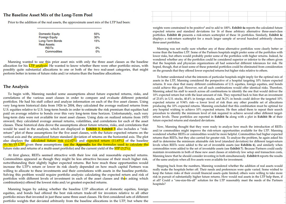
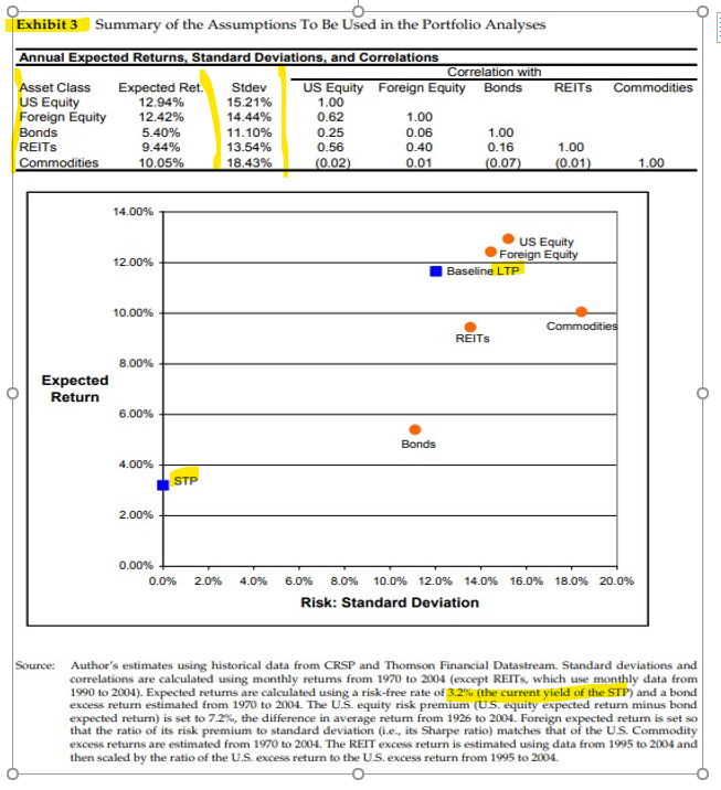
The Baseline Asset Mix of the Long-Term Pool Prior to the addition of the real assets, the approximate asset mix of the LTP had been: 55% 30% weights were constrained to be positive and to add to 100%. Exhibit 4a reports the calculated future expected returns and standard deviations for 16 of these arbitrary alternative three-asset-class portfolios. Exhibit 4b presents a risk-return scatterplot of these 16 portfolios. Similarly, Exhibit 4 displays a risk-return scatterplot for a much larger sample of several hundred arbitrarily chosen three-asset portfolios. Domestic Equity Foreign Equity Long-Term Bonds Real Assets REITS Commodities 15% 0% Manning wanted to use this prior asset mix with only the three asset classes as the baseline allocation for his LTP analysis. He wanted to know whether there were other portfolio mixes, with possibly quite substantial allocations to one or both of the two real-asset categories, that might perform better in terms of future risks and/or returns than the baseline allocations. The Analysis To begin with, Manning needed some assumptions about future expected returns, risks, and correlations of the various asset classes in order to compare and evaluate different potential portfolios. He had his staff collect and analyze information on each of the five asset classes. Using very long-term historical data from 1926 to 2004, they calculated the average realized returns from US, equities relative to U.S. long-term bonds in order to estimate the risk premium that equities had paid on average relative to bonds over this very long-term time horizon. Unfortunately, such very long-term data were not available for most asset classes. Using data on realized returns from 1970 onward, they calculated average annual retums, volatilities, and correlations for each of the asset classes. These historical data drove the assumptions about future returns, risks, and correlations that would be used in the analysis, which are displayed in Exhibit 3. Exhibit 3 also includes a "risk- return" plot of these assumptions for the five asset classes, with the future expected returns on the vertical axis and the annualized future standard deviation of retums on the horizontal axis. The plot also displays the calculated future risk (12.02%) and expected return (11.65%) of the baseline 55/30/15 LTP given these assumptions (see the Appendix for the formulas used to calculate the future risks and returns of a multi-asset portfolio) and the current yield of the STP (3.2%). Manning was not really sure whether any of these alternative portfolios were clearly better or worse than the baseline LTP. Some of the Partners hospitals might prefer some of the portfolios with lower risks, but others would probably prefer some of the portfolios with higher returns. Indeed, he wondered whether any of the portfolios could be considered superior or inferior to the others given that the hospitals and physician organizations all had somewhat different tolerances for risk. He hoped, though, that at least some of these potential portfolios could be eliminated from consideration on the grounds that they offered lower expected returns but higher risks relative to others. To better understand what the interests of particular hospitals might imply for the optimal mix of assets in the LTT, Manning considered the perspective of a hospital targeting 10% future expected returns. It was clear that many different combinations of U.S. equities, foreign equities, and bonds could achieve this goal. However, not all such combinations would offer identical risks. Therefore, Manning asked his staff to search across all combinations to identify the one that would deliver the 10% expected return but with the least amount of risk. They reported back to him that an investment of 23.4% in US stocks. 40.4% in foreign stocks and 36.2% in bonds could deliver the targeted 10% expected returns at 9.94% riska lower level of risk than any other possible set of allocations producing the 10% expected returns. Manning concluded that this combination must be optimal for any hospital wishing to achieve 10% expected returns. He then asked them to repeat their search procedure to identify the minimum level of risk required to achieve several other different target- retum levels. These portfolios are reported in Exhibit 5a along with a plot in Exhibit sb of their future expected returns and standard deviations Now, Manning thought that they were ready to analyze how much the introduction of REITS and/or commodities might improve the risk-retum opportunities available for the LTP. Manning wondered whether REITs or commodities would be more helpful. Commodities had higher expected returns than REITs, but they also carried far greater risk. To analyze the problem, he again asked his staff to determine the minimum attainable risk level (standard deviation) for different target-return levels when REITs were added to the set of investable assets (see Exhibits 6), and similarly when commodities were added to the set of investable assets (see Exhibit 7). Because Partners could easily maintain investments in both of these new asset classes at relatively low setup and transaction costs, Manning knew that he should consider investing in both simultaneously. Exhibit 8 reports the results of the same analysis when all five assets were available for investment. Stepping back from the numbers, Manning wondered whether the addition of real assets would really make the hospitals better off. Their needs and preferences were quite varied. Some wished to keep the future risks of their overall financial assets quite limited; others were willing to take more risk in pursuit of substantially higher future retums. How would real assets in the LTP help them, if at all? Could a "one-size-fits-all" solution for the LTP reasonably meet the needs of the Partners hospitals? At first glance, REITs seemed attractive with their low risk and reasonable expected retums. Commodities appeared as though they might be less attractive because of their much higher risk, notwithstanding their slightly higher expected returns. But how much these opportunities would increase the LTP's return or lower its risk clearly depended on how much capital Partners was willing to allocate to these investments and their correlations with assets in the baseline portfolio Solving this problem would require portfolio analysis: calculating the expected return and risk of portfolios with different levels of investment in each of the asset classes and then asking which combination(s) offered the lowest risks and/or greatest expected returns Manning began by asking whether the baseline LTP allocation of domestic equities, foreign equities, and bonds had offered the best risk-retum trade-off for investors relative to all other portfolio mixes that invested in just these same three asset classes. He first considered sets of different portfolio weights that deviated arbitrarily from the baseline allocations in the LTP, but where the Exhibit 3 Summary of the Assumptions To Be Used in the Portfolio Analyses REITs Commodities Annual Expected Returns, Standard Deviations, and Correlations Correlation with Asset Class Expected Ret. Stdev US Equity Foreign Equity Bonds US Equity 12.94% 15.21% 1.00 Foreign Equity 12.42% 14.44% 0.62 1.00 Bonds 5.40% 11.10% 0.25 0.06 1.00 REITS 9.44% 13.54% 0.56 0.40 0.16 Commodities 10.05% 18.43% (0.02) 0.01 (0.07) 1.00 (0.01) 1.00 14.00% US Equity Foreign Equity 12.00% Baseline LTP 10.00% Commodities REITS 8.00% Expected Return 6.00% Bonds 4.00% 2.00% 0.00% 0.0% 2.0% 4.0% 16.0% 18.0% 20.0% 6.0% 8.0% 0.0% 12.0% 14.0% Risk: Standard Deviation Source: Author's estimates using historical data from CRSP and Thomson Financial Datastream. Standard deviations and correlations are calculated using monthly retums from 1970 to 2004 (except REITs, which use monthly data from 1990 to 2004). Expected returns are calculated using a risk-free rate of 3.2% (the current yield of the STP) and a bond excess return estimated from 1970 to 2004. The U.S. equity risk premium (U.S. equity expected return minus bond expected return) is set to 7.2%, the difference in average return from 1926 to 2004. Foreign expected retum is set so that the ratio of its risk premium to standard deviation (ie, its Sharpe ratio) matches that of the US. Commodity excess returns are estimated from 1970 to 2004. The REIT excess return is estimated using data from 1995 to 2004 and then scaled by the ratio of the U.S. excess return to the US. excess return from 1995 to 2004. The Baseline Asset Mix of the Long-Term Pool Prior to the addition of the real assets, the approximate asset mix of the LTP had been: 55% 30% weights were constrained to be positive and to add to 100%. Exhibit 4a reports the calculated future expected returns and standard deviations for 16 of these arbitrary alternative three-asset-class portfolios. Exhibit 4b presents a risk-return scatterplot of these 16 portfolios. Similarly, Exhibit 4 displays a risk-return scatterplot for a much larger sample of several hundred arbitrarily chosen three-asset portfolios. Domestic Equity Foreign Equity Long-Term Bonds Real Assets REITS Commodities 15% 0% Manning wanted to use this prior asset mix with only the three asset classes as the baseline allocation for his LTP analysis. He wanted to know whether there were other portfolio mixes, with possibly quite substantial allocations to one or both of the two real-asset categories, that might perform better in terms of future risks and/or returns than the baseline allocations. The Analysis To begin with, Manning needed some assumptions about future expected returns, risks, and correlations of the various asset classes in order to compare and evaluate different potential portfolios. He had his staff collect and analyze information on each of the five asset classes. Using very long-term historical data from 1926 to 2004, they calculated the average realized returns from US, equities relative to U.S. long-term bonds in order to estimate the risk premium that equities had paid on average relative to bonds over this very long-term time horizon. Unfortunately, such very long-term data were not available for most asset classes. Using data on realized returns from 1970 onward, they calculated average annual retums, volatilities, and correlations for each of the asset classes. These historical data drove the assumptions about future returns, risks, and correlations that would be used in the analysis, which are displayed in Exhibit 3. Exhibit 3 also includes a "risk- return" plot of these assumptions for the five asset classes, with the future expected returns on the vertical axis and the annualized future standard deviation of retums on the horizontal axis. The plot also displays the calculated future risk (12.02%) and expected return (11.65%) of the baseline 55/30/15 LTP given these assumptions (see the Appendix for the formulas used to calculate the future risks and returns of a multi-asset portfolio) and the current yield of the STP (3.2%). Manning was not really sure whether any of these alternative portfolios were clearly better or worse than the baseline LTP. Some of the Partners hospitals might prefer some of the portfolios with lower risks, but others would probably prefer some of the portfolios with higher returns. Indeed, he wondered whether any of the portfolios could be considered superior or inferior to the others given that the hospitals and physician organizations all had somewhat different tolerances for risk. He hoped, though, that at least some of these potential portfolios could be eliminated from consideration on the grounds that they offered lower expected returns but higher risks relative to others. To better understand what the interests of particular hospitals might imply for the optimal mix of assets in the LTT, Manning considered the perspective of a hospital targeting 10% future expected returns. It was clear that many different combinations of U.S. equities, foreign equities, and bonds could achieve this goal. However, not all such combinations would offer identical risks. Therefore, Manning asked his staff to search across all combinations to identify the one that would deliver the 10% expected return but with the least amount of risk. They reported back to him that an investment of 23.4% in US stocks. 40.4% in foreign stocks and 36.2% in bonds could deliver the targeted 10% expected returns at 9.94% riska lower level of risk than any other possible set of allocations producing the 10% expected returns. Manning concluded that this combination must be optimal for any hospital wishing to achieve 10% expected returns. He then asked them to repeat their search procedure to identify the minimum level of risk required to achieve several other different target- retum levels. These portfolios are reported in Exhibit 5a along with a plot in Exhibit sb of their future expected returns and standard deviations Now, Manning thought that they were ready to analyze how much the introduction of REITS and/or commodities might improve the risk-retum opportunities available for the LTP. Manning wondered whether REITs or commodities would be more helpful. Commodities had higher expected returns than REITs, but they also carried far greater risk. To analyze the problem, he again asked his staff to determine the minimum attainable risk level (standard deviation) for different target-return levels when REITs were added to the set of investable assets (see Exhibits 6), and similarly when commodities were added to the set of investable assets (see Exhibit 7). Because Partners could easily maintain investments in both of these new asset classes at relatively low setup and transaction costs, Manning knew that he should consider investing in both simultaneously. Exhibit 8 reports the results of the same analysis when all five assets were available for investment. Stepping back from the numbers, Manning wondered whether the addition of real assets would really make the hospitals better off. Their needs and preferences were quite varied. Some wished to keep the future risks of their overall financial assets quite limited; others were willing to take more risk in pursuit of substantially higher future retums. How would real assets in the LTP help them, if at all? Could a "one-size-fits-all" solution for the LTP reasonably meet the needs of the Partners hospitals? At first glance, REITs seemed attractive with their low risk and reasonable expected retums. Commodities appeared as though they might be less attractive because of their much higher risk, notwithstanding their slightly higher expected returns. But how much these opportunities would increase the LTP's return or lower its risk clearly depended on how much capital Partners was willing to allocate to these investments and their correlations with assets in the baseline portfolio Solving this problem would require portfolio analysis: calculating the expected return and risk of portfolios with different levels of investment in each of the asset classes and then asking which combination(s) offered the lowest risks and/or greatest expected returns Manning began by asking whether the baseline LTP allocation of domestic equities, foreign equities, and bonds had offered the best risk-retum trade-off for investors relative to all other portfolio mixes that invested in just these same three asset classes. He first considered sets of different portfolio weights that deviated arbitrarily from the baseline allocations in the LTP, but where the Exhibit 3 Summary of the Assumptions To Be Used in the Portfolio Analyses REITs Commodities Annual Expected Returns, Standard Deviations, and Correlations Correlation with Asset Class Expected Ret. Stdev US Equity Foreign Equity Bonds US Equity 12.94% 15.21% 1.00 Foreign Equity 12.42% 14.44% 0.62 1.00 Bonds 5.40% 11.10% 0.25 0.06 1.00 REITS 9.44% 13.54% 0.56 0.40 0.16 Commodities 10.05% 18.43% (0.02) 0.01 (0.07) 1.00 (0.01) 1.00 14.00% US Equity Foreign Equity 12.00% Baseline LTP 10.00% Commodities REITS 8.00% Expected Return 6.00% Bonds 4.00% 2.00% 0.00% 0.0% 2.0% 4.0% 16.0% 18.0% 20.0% 6.0% 8.0% 0.0% 12.0% 14.0% Risk: Standard Deviation Source: Author's estimates using historical data from CRSP and Thomson Financial Datastream. Standard deviations and correlations are calculated using monthly retums from 1970 to 2004 (except REITs, which use monthly data from 1990 to 2004). Expected returns are calculated using a risk-free rate of 3.2% (the current yield of the STP) and a bond excess return estimated from 1970 to 2004. The U.S. equity risk premium (U.S. equity expected return minus bond expected return) is set to 7.2%, the difference in average return from 1926 to 2004. Foreign expected retum is set so that the ratio of its risk premium to standard deviation (ie, its Sharpe ratio) matches that of the US. Commodity excess returns are estimated from 1970 to 2004. The REIT excess return is estimated using data from 1995 to 2004 and then scaled by the ratio of the U.S. excess return to the US. excess return from 1995 to 2004