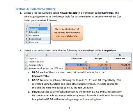
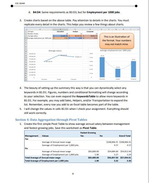
Section 3: Dynamic Summary 1. Create a job lookup table called KeywordsTable in a worksheet called Keywords. This table is going to serve as the lookup table for data validation of another worksheet (see bullet point number 2 below). 1 Keyword 2 Education 3 Assistants 4 Engineering 5 Computer This is an illustration of the format. Your numbers may not match mine. 29 23 $ 2. Create a job comparison table like the following in a worksheet called Comparison: B D 1 Keyword: Education Analyst Computer 2 Number of jobs 12 3 Average salary 61.102.76 S 84,747.50 $ 78,691.74 4. Average employment per 1000 jobs: $ 5.10 $ 2.18 S 4.12 a. B1:01: each of them is a drop down list box with values from the KeywordsTable. b. B2:02: Number of jobs mentioning the term in B1, C1, and D1 respectively. This is created using COUNTIF and table structured reference. The data source for this and the next two bullet points is the Full List table. C B3:03. Average salary of jobs mentioning the term in B1, C1 and D1 respectively. Be sure to use table structured reference in your formula. Conditional formatting is applied to B3:03 with max being orange and min being blue. 3 CIS 2640 d. B4:04: Same requirements as B3:03, but for Employment per 1000 jobs 3. Create charts based on the above table. Pay attention to details in the charts. You must replicate every detail in the charts. This helps you review a few things about charts. Job het och Are BUS 10 12 N30 28 This is an illustration of the format. Your numbers may not match mine. Average Average employment per 1000 13 SI 21 22 23 4. The beauty of setting up the summary this way is that you can dynamically select any keywords in B1:01. Figures, numbers and conditional formatting will change according to your selection. You can even expand the KeywordsTable to allow more keywords in B1:01. For example, you may add Sales, Helpers, and/or Transportation to expand the list. Remember, every row you add to an Excel table becomes part of the table. 5. I will change the values in cells B1:01 when I check your assignment. Everything should still work correctly. Section 4: Data Aggregation through Pivot Tables 1. Create the first simple Pivot Table to show average annual salary between management and fastest growing jobs. Save this worksheet as Pivot Table. Fastest growing Management Values Yes No Grand Total Yes Average of Annual mean w $108.906 41 S108 90641 Average of Employment per 1,000 jobs 457 No Average of Annual meanwege $65.600.00 $54,684.60 $54,913:44 Average of Employment per 1,000 jobs 1.90 3.22 3.24 Total Average of Annual mean wape $65,000.00 $56,857.95 $7,056.01 Total Average of Employment per 1.000 jobs 1.90 3:32 3.30 45 Section 3: Dynamic Summary 1. Create a job lookup table called KeywordsTable in a worksheet called Keywords. This table is going to serve as the lookup table for data validation of another worksheet (see bullet point number 2 below). 1 Keyword 2 Education 3 Assistants 4 Engineering 5 Computer This is an illustration of the format. Your numbers may not match mine. 29 23 $ 2. Create a job comparison table like the following in a worksheet called Comparison: B D 1 Keyword: Education Analyst Computer 2 Number of jobs 12 3 Average salary 61.102.76 S 84,747.50 $ 78,691.74 4. Average employment per 1000 jobs: $ 5.10 $ 2.18 S 4.12 a. B1:01: each of them is a drop down list box with values from the KeywordsTable. b. B2:02: Number of jobs mentioning the term in B1, C1, and D1 respectively. This is created using COUNTIF and table structured reference. The data source for this and the next two bullet points is the Full List table. C B3:03. Average salary of jobs mentioning the term in B1, C1 and D1 respectively. Be sure to use table structured reference in your formula. Conditional formatting is applied to B3:03 with max being orange and min being blue. 3 CIS 2640 d. B4:04: Same requirements as B3:03, but for Employment per 1000 jobs 3. Create charts based on the above table. Pay attention to details in the charts. You must replicate every detail in the charts. This helps you review a few things about charts. Job het och Are BUS 10 12 N30 28 This is an illustration of the format. Your numbers may not match mine. Average Average employment per 1000 13 SI 21 22 23 4. The beauty of setting up the summary this way is that you can dynamically select any keywords in B1:01. Figures, numbers and conditional formatting will change according to your selection. You can even expand the KeywordsTable to allow more keywords in B1:01. For example, you may add Sales, Helpers, and/or Transportation to expand the list. Remember, every row you add to an Excel table becomes part of the table. 5. I will change the values in cells B1:01 when I check your assignment. Everything should still work correctly. Section 4: Data Aggregation through Pivot Tables 1. Create the first simple Pivot Table to show average annual salary between management and fastest growing jobs. Save this worksheet as Pivot Table. Fastest growing Management Values Yes No Grand Total Yes Average of Annual mean w $108.906 41 S108 90641 Average of Employment per 1,000 jobs 457 No Average of Annual meanwege $65.600.00 $54,684.60 $54,913:44 Average of Employment per 1,000 jobs 1.90 3.22 3.24 Total Average of Annual mean wape $65,000.00 $56,857.95 $7,056.01 Total Average of Employment per 1.000 jobs 1.90 3:32 3.30 45