Signal analysis,

For the Matlab code given below,

it is required to 1- add the settling time function to get the settling time at each alpha,

                               2-fix the 3dB line (which equal to (1/root(2))* magnitude) to be shown correctly

in order to complete the following table

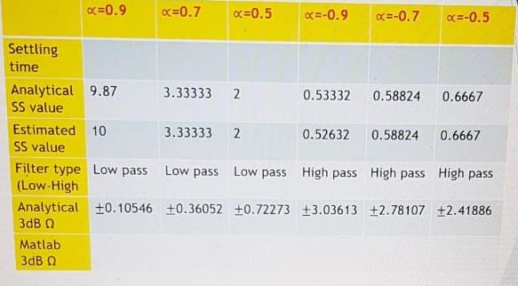
***the settling time is the time required for the step response to reach and stay within a range of 5% of the final steady-state value. It can be used to evaluate system speed (higher settling time corresponds to a slower system). Use Matlab to find the settling time for this case***

The Matlab code:

clc; close all; clear; syms w n z; %creating symbolic variables w,n,z wr = -pi:0.1:pi; %range of w for magnitude and phase plot nr = 0:40; %n range for plotting the signal in time domain alpha_arr = [0.9 0.7 0.5 -0.9 -0.7 -0.5]; %defining array for required alpha valuesfor i = 1:length(alpha_arr)    figure; %opening a new figure    alpha = alpha_arr(i);    x = alpha^n; %defining the function x(n)    subplot 221    stem(nr,subs(x,n,nr)); % for plotting x(n)    hold on;    plot(nr,0.05*ones(1,length(nr)),'r'); %plotting the upperline for 5% settling time    plot(nr,-0.05*ones(1,length(nr)),'r'); %plotting the downline for 5% settling time    hold off;    title(["Impulse response for alpha = " alpha]);    legend("x(n)","5% value");    xlabel("n");    ylabel("h(n)");    Zx = ztrans(x); %for freq response we first need to find the z transform    Step_z = Zx*1/(1-z^-1); %z transform of TF multiplied with z transform of step input    Step_n = iztrans(Step_z);    %finding the step response    subplot 222    stem(nr,subs(Step_n,n,nr));    %plotting the step response    title(["Step Response for alpha = " alpha]);    xlabel("n");    ylabel("S(n)");    X_w = subs(Zx,z,exp(1i*w));   % Put z = exp(jw) to find the frequency response    subplot 223    plot(wr,(abs(subs(X_w,w,wr)))); %plotting the magnitude response    hold on;    plot(wr,-3*ones(1,length(wr)),'r');    %-3dB line    hold off;    title(["Magnitude plot (in dB) for alpha = " alpha]);    legend("Magnitude plot","-3dB line");    xlabel("w");    ylabel("|H(e^jw)|");    subplot 224    plot(wr,180*angle(subs(X_w,w,wr))/pi); %plotting the phase response    title(["Phase Plot for alpha = " alpha]);    xlabel("w");    ylabel("<[H(e^jw)]"); end

Settling time x=0.9 Analytical 9.87 SS value Estimated 10 SS value Matlab 3dB x=0.7 x=0.5 3.33333 2 3.33333 2 Filter type Low pass Low pass Low pass (Low-High Analytical 0.10546 +0.36052 +0.72273 3dB x=-0.9 x=-0.7 x=-0.5 0.53332 0.58824 0.6667 0.52632 0.58824 0.6667 High pass High pass High pass +3.03613 +2.78107 +2.41886