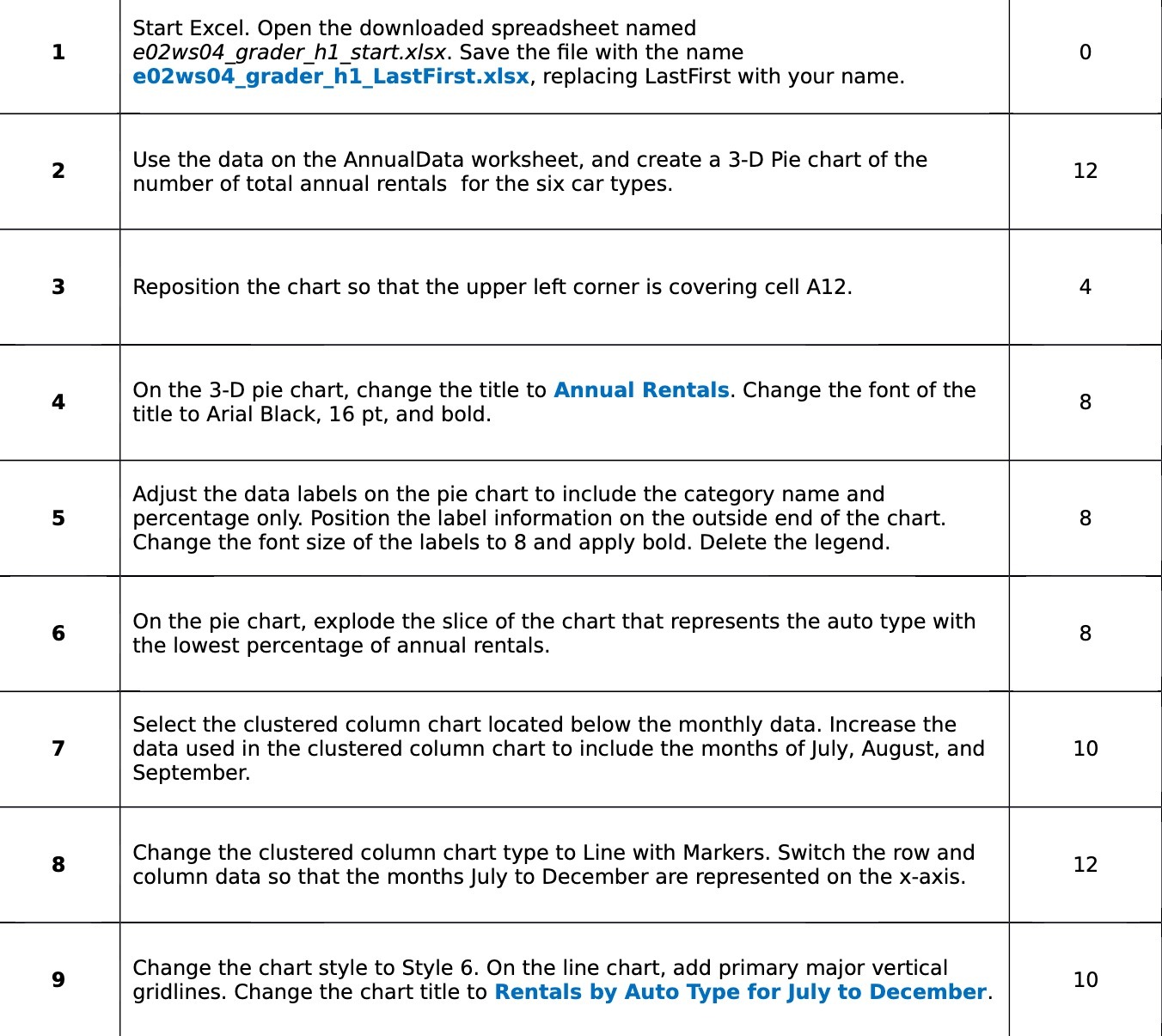
Start Excel. Open the downloaded spreadsheet named 602W504 _grader_h1_start.xlsx. Save the le with the name e02wso4_grader_h1_LastFirst.xlsx. replacing LastFirst with your name. Use the data on the AnnualData worksheet. and create a 3-D Pie chart of the number of total annual rentals for the six car types. Reposition the chart so that the upper left corner is covering cell A12. On the 3-D pie chart. change the title to Annual Rentals. Change the font of the title to Arial Black, 16 pt, and bold. Adjust the data labels on the pie chart to include the category name and percentage only. Position the label information on the outside end of the chart. Change the font size of the labels to 8 and apply bold. Delete the legend. On the pie chart, explode the slice of the chart that represents the auto type with the lowest percentage of annual rentals. Select the clustered column chart located below the monthly data. Increase the data used in the clustered column chart to include the months ofJuly. August, and September. Change the clustered column chart type to Line with Markers. Switch the row and column data so that the monthsjuly to December are represented on the x-axis. Change the chart style to Style 6. 0n the line chart, add primary major vertical gridlines. Change the chart title to Rentals by Auto Type for july to December. 12 10 12 10