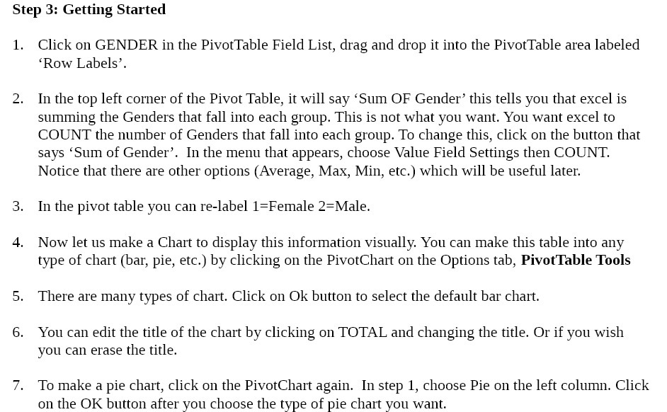
Step 3: Getting Started 1. Click on GENDER in the PivotTable Field List, drag and drop it into the PivotTable area labeled 'Row Labels'. 2. In the top left corner of the Pivot Table, it will say 'Sum OF Gender' this tells you that excel is summing the Genders that fall into each group. This is not what you want. You want excel to COUNT the number of Genders that fall into each group. To change this, click on the button that says 'Sum of Gender'. In the menu that appears, choose Value Field Settings then COUNT. Notice that there are other options (Average, Max, Min, etc.) which will be useful later. 3. In the pivot table you can re-label 1=Female 2=Male. 4. Now let us make a Chart to display this information visually You can make this table into any type of chart (bar, pie, etc.) by clicking on the PivotChart on the Options tab, Pivot'Iable Tools 5. There are many types of chart. Click on Ok button to select the default bar chart. 6. You can edit the title of the chart by clicking on TOTAL and changing the title. Or if you wish you can erase the title. 7. To make a pie chart, click on the PivotChart again. In step 1, choose Pie on the left column. Click on the OK button after you choose the type of pie chart you want