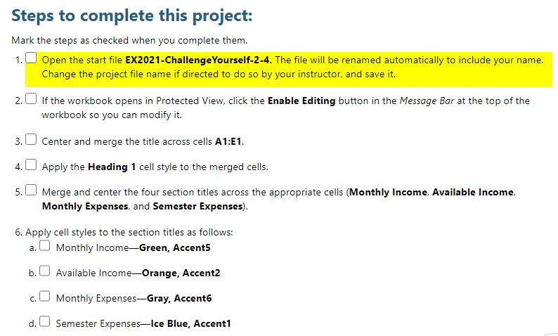
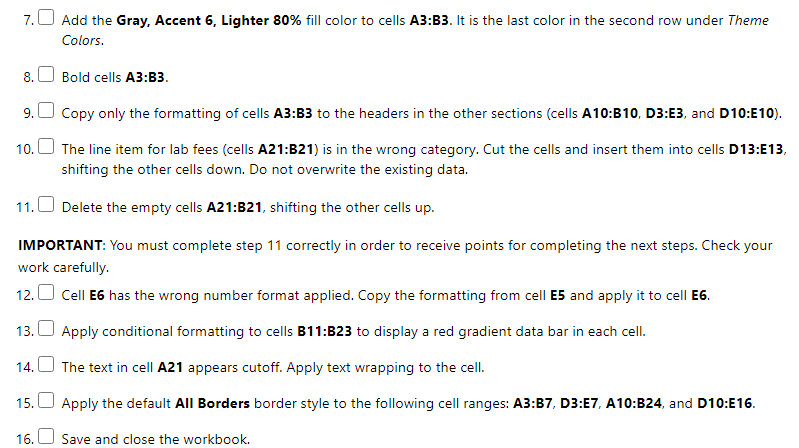
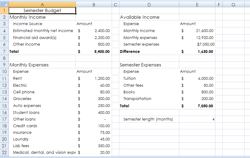
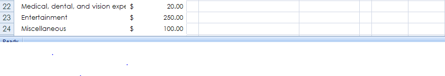
Steps to complete this project: Mark the steps as checked when you complete them. 1. Open the start file EX2021-ChallengeYourself-2-4. The file will be renamed automatically to include your name. Change the project file name if directed to do so by your instructor, and save it. 2. If the workbook opens in Protected View, click the Enable Editing button in the Message Bar at the top of the workbook so you can modify it. 3. Center and merge the title across cells A1:E1. 4. Apply the Heading 1 cell style to the merged cells. 5. Merge and center the four section titles across the appropriate cells (Monthly Income, Available Income, Monthly Expenses, and Semester Expenses). 6. Apply cell styles to the section titles as follows: a. Monthly Income-Green, Accent5 b. Available Income-Orange, Accent2 c. Monthly Expenses-Gray, Accent6 d. Semester Expenses-Ice Blue, Accent17. Add the Gray, Accent 6, Lighter 80% fill color to cells A3:B3. It is the last color in the second row under Theme Colors. 8. Bold cells A3:63. 9. Copy only the formatting of cells A3:B3 to the headers in the other sections (cells A10:B10, D3:E3, and D 10:E10). 10. The line item for lab fees (cells A21:B21) is in the wrong category. Cut the cells and insert them into cells D13:E13, shifting the other cells down. Do not overwrite the existing data. 11. Delete the empty cells A21:B21, shifting the other cells up. IMPORTANT: You must complete step 11 correctly in order to receive points for completing the next steps. Check your work carefully. 12. Cell E6 has the wrong number format applied. Copy the formatting from cell ES and apply it to cell E6. 13. Apply conditional formatting to cells B11:823 to display a red gradient data bar in each cell. 14. ) The text in cell A21 appears cutoff. Apply text wrapping to the cell. 15. Apply the default All Borders border style to the following cell ranges: A3:B7, D3:E7, A10:B24, and D10:E16. 16. Save and close the workbook.A B C D E F G Semester Budget 2 Monthly Income Available Income 3 Income Source Amount Expense Amount 4 Estimated monthly net income $ 2,400.00 Monthly Income 21,600.00 to to 5 Financial aid award (s) 2,200.00 Monthly expenses 12,920.00 Other income 800.00 Semester expenses $7,050.00 Total 5,400.00 Difference 1,630.00 8 9 Monthly Expenses Semester Expenses 10 Expense Amount Expense Amount 11 Rent 1,200.00 Tuition $ 6,000.00 12 Electric 60.00 Other fees 50.00 13 Cell phone 80.00 Books 800.00 14 Groceries 300.00 Transportation 200.00 15 Auto expenses 250.00 Total 7,050.00 16 Student loans 400.00 17 Other loans Semester length (months) 4 18 Credit cards 100.00 19 Insurance 75.00 20 Laundry 45.00 21 Lab fees 350.00 22 Medical, dental, and vision expe 20.00\f