Summarize and evaluate the model

1)Is the signs consistent with the theories or sense?

2)Evaluate each parameter individual applying T-test and P-value

3)R square coeffecient whether it is high or not and what R square number indicates for?

4)Is the estimated parameter significant with 1%,5% or 10% etc,,,,expalin the intercept and the slope?

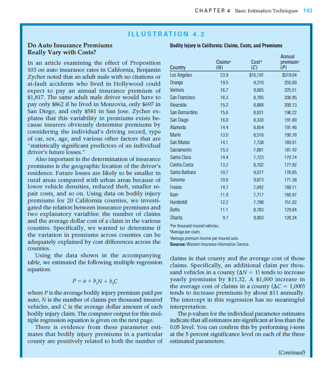
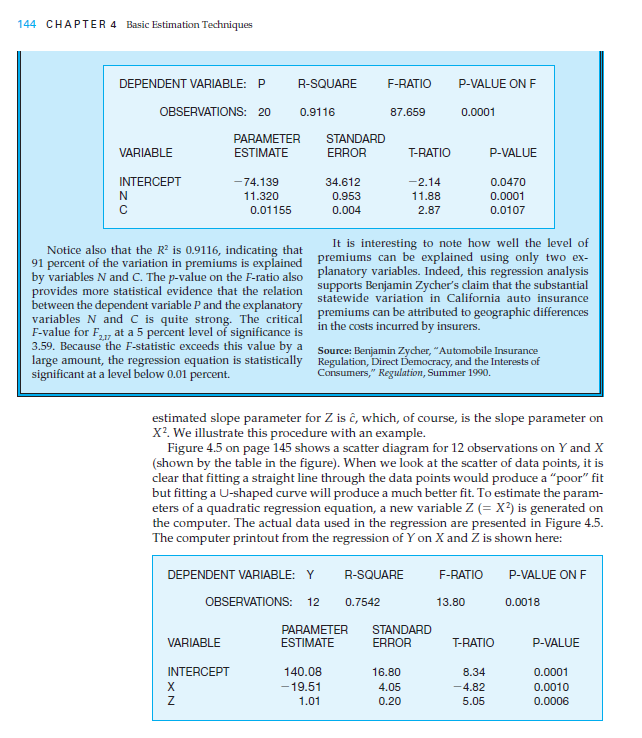
CHAPTER 4 Basic Estimation Techniques 143 23.9 19.5 16.3 15.2 15.6 16.0 14.4 ILLUSTRATION 4.2 Do Auto Insurance Premiums Bodily Injury in California: Claims, Costs, and Premiums Really Vary with Costs? Annual In an article examining the effect of Proposition Claims Cost" premium (N) Country (C) (P) 103 on auto insurance rates in California, Benjamin Zycher noted that an adult male with no citations or Los Angeles $10,197 $319.04 at-fault accidents who lived in Hollywood could Orange 9,270 255.00 expect to pay an annual insurance premium of Ventura 16.7 9,665 225.51 $1,817. The same adult male driver would have to San Francisco 8,705 208.95 pay only $862 if he lived in Monrovia, only $697 in Riverside 8,888 200.13 San Diego, and only $581 in San Jose. Zycher ex San Bernardino 8,631 196 22 plains that this variability in premiums exists be San Diego 8,330 191.80 cause insurers obviously determine premiums by Alameda 8,654 191.46 considering the individual's driving record, type Marin 13.0 8,516 190.78 of car, sex, age, and various other factors that are San Mateo 7,738 189.01 "statistically significant predictors of an individual Sacramento 7,881 181.42 driver's future losses." Also important in the determination of insurance Santa Clara 7,723 179.74 premiums is the geographic location of the driver's Contra Costa 8,702 17792 residence. Future losses are likely to be smaller in Santa Barbara 9,077 176.65 rural areas compared with urban areas because of Sonoma 9,873 17138 lower vehicle densities, reduced theft, smaller re Fresno 7,842 168.11 pair costs, and so on. Using data on bodily injury Kam 7,717 160.97 premiums for 20 California counties, we investi- Humboldt 7,798 151.02 gated the relation between insurance premiums and Butte 8,783 129.84 two explanatory variables: the number of claims 9,803 and the average dollar cost of a claim in the various counties. Specifically, we wanted to determine if Per thousand insured vehicles. "Average per claim the variation in premiums across counties can be Average premium income per insured auto. adequately explained by cost differences across the Source: Western Insurance Information Service. counties. Using the data shown in the accompanying claims in that county and the average cost of those table, we estimated the following multiple regression claims. Specifically, an additional claim per thou- equation: sand vehicles in a county (AN = 1) tends to increase P= a + b + b c yearly premiums by $11.32. A $1,000 increase in the average cost of claims in a county (AC = 1,000) where P is the average bodily injury premium paid per tends to increase premiums by about $11 annually. auto, N is the number of claims per thousand insured The intercept in this regression has no meaningful vehicles, and is the average dollar amount of each interpretation. bodily injury claim. The computer output for this mul The p-values for the individual parameter estimates tiple regression equation is given on the next page. indicate that all estimates are significant at less than the There is evidence from these parameter esti- 0.05 level. You can confirm this by performing t-tests mates that bodily injury premiums in a particular at the 5 percent significance level on each of the three county are positively related to both the number of estimated parameters. (Continued) 14.1 15.3 14.4 13.2 10.7 10.6 14.7 11.9 122 11.1 Shasta 9.7 126.34 144 CHAPTER 4 Basic Estimation Techniques DEPENDENT VARIABLE: P R-SQUARE F-RATIO P-VALUE ON F 87.659 0.0001 T-RATIO P-VALUE OBSERVATIONS: 20 0.9116 PARAMETER STANDARD VARIABLE ESTIMATE ERROR INTERCEPT - 74.139 34.612 N 11.320 0.953 0.01155 0.004 -2.14 11.88 2.87 0.0470 0.0001 0.0107 Notice also that the R is 0.9116, indicating that It is interesting to note how well the level of 91 percent of the variation in premiums is explained premiums can be explained using only two ex- by variables N and C. The p-value on the F-ratio also planatory variables. Indeed, this regression analysis provides more statistical evidence that the relation supports Benjamin Zycher's claim that the substantial between the dependent variable P and the explanatory statewide variation in California auto insurance variables N and C is quite strong. The critical premiums can be attributed to geographic differences F-value for F, at a 5 percent level of significance is in the costs incurred by insurers. 3.59. Because the F-statistic exceeds this value by a Source: Benjamin Zycher, Automobile Insurance large amount, the regression equation is statistically Regulation, Direct Democracy, and the Interests of significant at a level below 0.01 percent. Consumers," Regulation, Summer 1990. estimated slope parameter for Z is , which, of course, is the slope parameter on X? We illustrate this procedure with an example. Figure 4.5 on page 145 shows a scatter diagram for 12 observations on Y and X (shown by the table in the figure). When we look at the scatter of data points, it is clear that fitting a straight line through the data points would produce a "poor" fit but fitting a U-shaped curve will produce a much better fit. To estimate the param- eters of a quadratic regression equation, a new variable Z (= x2) is generated on the computer. The actual data used in the regression are presented in Figure 4.5. The computer printout from the regression of Yon X and Z is shown here: R-SQUARE F-RATIO P-VALUE ON F DEPENDENT VARIABLE: Y OBSERVATIONS: 12 0.7542 13.80 0.0018 VARIABLE PARAMETER ESTIMATE STANDARD ERROR T-RATIO P-VALUE INTERCEPT Z 140.08 - 19.51 1.01 16.80 4.05 0.20 8.34 -4.82 5.05 0.0001 0.0010 0.0006