

Question: Supply Chain Management: A. Using a spreadsheet model, solve the demand allocation model for TelecomOne assuming that all its facilities are already open (i.e., find
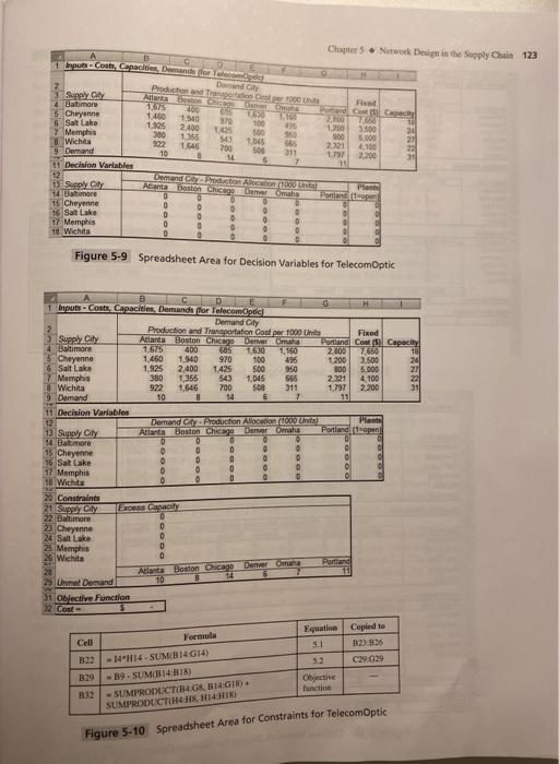
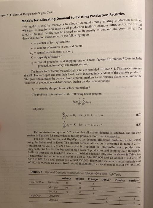
Chapter 5 Network Design in the Supply Chain 123 Red F Input Costs Capacities Demande force.com.pe 2 Prediction and Transportation or Dend Supply City & Babimore 15675 TOO 5 Cheyenne 1,460 1940 970 6. Salt Lake 1.926 100 095 2.400 1.425 7 Memphis 380 500 10 1355 545 922 1646 7,045 65 700 Go 10 311 14 5 1 11 Decision Variables 12 13 Supply City Acante Bottomas 14 Balmore 0 15 Cheyenne 0 16. Salt Lake 0 0 0 0 17 Memphis 0 0 0 16 Wichita 0 0 0 8 Wichita 9 Demand 2000 1.200 000 2.321 1757 10 31.500 5.000 4,100 2.200 Potland (traper Figure 5-9 Spreadsheet Area for Decision Variables for TelecomOptic B DE Input Costs. Capacitles, Demand for Telecom G Demand City Production and Transportation Cost per 1000 Uhits Fixed Supply City Atlanta Boston Chic Denver Omaha Portland Cow () Capacity 4 Baltimore 1.675 400 685 1,630 1150 2006 7,650 tel 5 Cheyenne 1.460 1,940 920 100 496 1.200 3.500 24 5. Salt Lake 1,925 2,400 1425 500 950 300 5.000 Memphis 350 1.355 1,045 566 2221 4.100 8 Wichita 922 1,646 700 SOS 311 1.797 2.200 31 9 Demand 10 B 14 6 7 11 11 Decision Variables 12 Demand Cy Production Allocation Unit Plants 13 Supply City Allants Boston Chicago Denver Omaha Portland Cropen! 14 Bat more O 0 15 Cheyenne 0 15. Sat Lake 0 ol 17 Memphis 0 10 Wichita 20 Constraints 21 Suppy City des Capacity 22 Baltimore 23 Cheyenne 0 24 Salt Lake 0 25 Memphis 26 Wichita 0 Denver Omaha Portand Atlanta Boston Chicago 29 Uhine Demand 31 Objective Function 22 Gost- DOO DODOC OBOR DOO 1 10 Cell R22 Formula -14H14 - SUMB14 G14) - B9. SUMB4-815) SUMPRODLICTGS. B14 GIS). SLMPRODUCTCHH, H14118) Equation Copled to 5:1 5.2 C29.29 Objective function B29 RUZ Figure 5-10 Spreadsheet Area for constraints for TelecomOptic apter 5 Network Design in the Supply Chain Models for Allocating Demand to Existing Production Facilities This model is used by managers to allocate demand among existing production facilities Whereas the location and capacity of production facilities changes infrequently, the demand allocated to each facility can be altered more frequently as demand and costs change. The demand allocation model requires the following inputs: n = number of factory locations m = number of markets or demand points D = annual demand from market K = capacity of factory i = cost of producing and shipping one unit from factory i to market (cost includes production, inventory, and transportation) The inputs for TelecomOne and High Optic are provided in Table 5-1. This model assumes that all plants are open and thus their fixed cost is incurred independent of the quantity produced The goal is to allocate the demand from different markets to the various plants to minimize the total cost of production and distribution. Define the decision variables: - quantity shipped from factory i to market The problem is formulated as the following linear program: Min Set subject to x =D for - I.....m (5.7) SK for i=1.....n (5.8 The constraints in Equation 5.7 ensure that all market demand is satisfied, and the con straints in Equation 5.8 ensure that no factory produces more than its capacity. For both TelecomOne and HighOptic, the demand allocation problem can be solved using the Solver tool in Excel. The optimal demand allocation is presented in Table 5-2 (sec spreadsheet Figures 5.9 to 12). Observe that it is optimal for TelecomOne not to produce any thing in the Wichita facility because of high costs of production and shipping even though the facility is open and the fixed cost is incurred. With the demand allocation as shown in Table 5-2. TelecomOne incurs an annual variable cost of $14,886,000 and an annual fixed cost of $13.950,000, for a total annual cost of $28.836,000. High Optic incurs an annual variable cost of S12.865,000 and an annual fixed cost of $8,500,000, for a total annual cost of $21,365,000 Portland TABLE 5-2 Optimal Demand Allocation for TelecomOne and High Optic Atlanta Boston Chicago Denver Omaha TelecomOne Baltimore 0 8 2 Memphis 10 0 12 Wichita 0 0 High Optik Cheyenne 0 0 Salt Lake 6 7 0 Chapter 5 Network Design in the Supply Chain 123 Red F Input Costs Capacities Demande force.com.pe 2 Prediction and Transportation or Dend Supply City & Babimore 15675 TOO 5 Cheyenne 1,460 1940 970 6. Salt Lake 1.926 100 095 2.400 1.425 7 Memphis 380 500 10 1355 545 922 1646 7,045 65 700 Go 10 311 14 5 1 11 Decision Variables 12 13 Supply City Acante Bottomas 14 Balmore 0 15 Cheyenne 0 16. Salt Lake 0 0 0 0 17 Memphis 0 0 0 16 Wichita 0 0 0 8 Wichita 9 Demand 2000 1.200 000 2.321 1757 10 31.500 5.000 4,100 2.200 Potland (traper Figure 5-9 Spreadsheet Area for Decision Variables for TelecomOptic B DE Input Costs. Capacitles, Demand for Telecom G Demand City Production and Transportation Cost per 1000 Uhits Fixed Supply City Atlanta Boston Chic Denver Omaha Portland Cow () Capacity 4 Baltimore 1.675 400 685 1,630 1150 2006 7,650 tel 5 Cheyenne 1.460 1,940 920 100 496 1.200 3.500 24 5. Salt Lake 1,925 2,400 1425 500 950 300 5.000 Memphis 350 1.355 1,045 566 2221 4.100 8 Wichita 922 1,646 700 SOS 311 1.797 2.200 31 9 Demand 10 B 14 6 7 11 11 Decision Variables 12 Demand Cy Production Allocation Unit Plants 13 Supply City Allants Boston Chicago Denver Omaha Portland Cropen! 14 Bat more O 0 15 Cheyenne 0 15. Sat Lake 0 ol 17 Memphis 0 10 Wichita 20 Constraints 21 Suppy City des Capacity 22 Baltimore 23 Cheyenne 0 24 Salt Lake 0 25 Memphis 26 Wichita 0 Denver Omaha Portand Atlanta Boston Chicago 29 Uhine Demand 31 Objective Function 22 Gost- DOO DODOC OBOR DOO 1 10 Cell R22 Formula -14H14 - SUMB14 G14) - B9. SUMB4-815) SUMPRODLICTGS. B14 GIS). SLMPRODUCTCHH, H14118) Equation Copled to 5:1 5.2 C29.29 Objective function B29 RUZ Figure 5-10 Spreadsheet Area for constraints for TelecomOptic apter 5 Network Design in the Supply Chain Models for Allocating Demand to Existing Production Facilities This model is used by managers to allocate demand among existing production facilities Whereas the location and capacity of production facilities changes infrequently, the demand allocated to each facility can be altered more frequently as demand and costs change. The demand allocation model requires the following inputs: n = number of factory locations m = number of markets or demand points D = annual demand from market K = capacity of factory i = cost of producing and shipping one unit from factory i to market (cost includes production, inventory, and transportation) The inputs for TelecomOne and High Optic are provided in Table 5-1. This model assumes that all plants are open and thus their fixed cost is incurred independent of the quantity produced The goal is to allocate the demand from different markets to the various plants to minimize the total cost of production and distribution. Define the decision variables: - quantity shipped from factory i to market The problem is formulated as the following linear program: Min Set subject to x =D for - I.....m (5.7) SK for i=1.....n (5.8 The constraints in Equation 5.7 ensure that all market demand is satisfied, and the con straints in Equation 5.8 ensure that no factory produces more than its capacity. For both TelecomOne and HighOptic, the demand allocation problem can be solved using the Solver tool in Excel. The optimal demand allocation is presented in Table 5-2 (sec spreadsheet Figures 5.9 to 12). Observe that it is optimal for TelecomOne not to produce any thing in the Wichita facility because of high costs of production and shipping even though the facility is open and the fixed cost is incurred. With the demand allocation as shown in Table 5-2. TelecomOne incurs an annual variable cost of $14,886,000 and an annual fixed cost of $13.950,000, for a total annual cost of $28.836,000. High Optic incurs an annual variable cost of S12.865,000 and an annual fixed cost of $8,500,000, for a total annual cost of $21,365,000 Portland TABLE 5-2 Optimal Demand Allocation for TelecomOne and High Optic Atlanta Boston Chicago Denver Omaha TelecomOne Baltimore 0 8 2 Memphis 10 0 12 Wichita 0 0 High Optik Cheyenne 0 0 Salt Lake 6 7 0
Step by Step Solution
There are 3 Steps involved in it

Get step-by-step solutions from verified subject matter experts