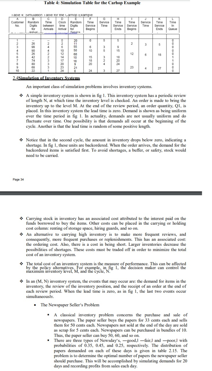
Table 4: Simulation Table for the Carhop Example Table 4: Simulation i apie for the Carnop Example A B D E F Customer Random Time Clock Random Time No. Digits between time Digits for Arrivals Arrival for Begins Aga L. Sandro G Service Time Service H 1 Time Time Service Service Ends Begins Service Time K Time Service Ends L. Time In Queue 0 5 5 2 3 5 2 3 4 5 6 0 2 6 10 12 6 10 3 5 9 15 12 6 26 98 90 26 42 74 80 68 22 18 20 11 55 50 68 10 16 9 21 6 2 4 4 2 2 3 3 3 1 15 18 20 3 2 18 20 24 0 0 0 0 0 1 1 0 0 0 8 9 10 23 23 24 27 24 3 27 2.4Simulation of Inventory Systems An important class of simulation problems involves inventory systems. A simple inventory system is shown in fig 1. This inventory system has a periodic review of length N, at which time the inventory level is checked. An order is made to bring the inventory up to the level M. At the end of the review period, an order quantity, Q1, is placed. In this inventory system the lead time is zero. Demand is shown as being uniform over the time period in fig 1. In actuality, demands are not usually uniform and do fluctuate over time. One possibility is that demands all occur at the beginning of the cycle. Another is that the lead time is random of some positive length. Notice that in the second cycle, the amount in inventory drops below zero, indicating a shortage. In fig 1, these units are backordered. When the order arrives, the demand for the backordered items is satisfied first. To avoid shortages, a buffer, or safety, stock would need to be carried. Page 34 * Carrying stock in inventory has an associated cost attributed to the interest paid on the funds borrowed to buy the items. Other costs can be placed in the carrying or holding cost column: renting of storage space, hiring guards, and so on. An alternative to carrying high inventory is to make more frequent reviews, and consequently, more frequent purchases or replenishments. This has an associated cost: the ordering cost. Also, there is a cost in being short. Larger inventories decrease the possibilities of shortages. These costs must be traded off in order to minimize the total cost of an inventory system. The total cost of an inventory system is the measure of performance. This can be affected by the policy alternatives. For example, in fig 1, the decision maker can control the maximum inventory level, M, and the cycle, N. . In an (M, N) inventory system, the events that may occur are: the demand for items in the inventory, the review of the inventory position, and the receipt of an order at the end of each review period. When the lead time is zero, as in fig 1, the last two events occur simultaneously. The Newspaper Seller's Problem A classical inventory problem concerns the purchase and sale of newspapers. The paper seller buys the papers for 33 cents each and sells them for 50 cents each. Newspapers not sold at the end of the day are sold as scrap for 5 cents each. Newspapers can be purchased in bundles of 10. Thus, the paper seller can buy 50, 60, and so on. There are three types of Newsday's, -good,l -fair, and --poor, with probabilities of 0.35, 0.45, and 0.25, respectively. The distribution of papers demanded on each of these days is given in table 2.15. The problem is to determine the optimal number of papers the newspaper seller should purchase. This will be accomplished by simulating demands for 20 days and recording profits from sales each day. Table 4: Simulation Table for the Carhop Example Table 4: Simulation i apie for the Carnop Example A B D E F Customer Random Time Clock Random Time No. Digits between time Digits for Arrivals Arrival for Begins Aga L. Sandro G Service Time Service H 1 Time Time Service Service Ends Begins Service Time K Time Service Ends L. Time In Queue 0 5 5 2 3 5 2 3 4 5 6 0 2 6 10 12 6 10 3 5 9 15 12 6 26 98 90 26 42 74 80 68 22 18 20 11 55 50 68 10 16 9 21 6 2 4 4 2 2 3 3 3 1 15 18 20 3 2 18 20 24 0 0 0 0 0 1 1 0 0 0 8 9 10 23 23 24 27 24 3 27 2.4Simulation of Inventory Systems An important class of simulation problems involves inventory systems. A simple inventory system is shown in fig 1. This inventory system has a periodic review of length N, at which time the inventory level is checked. An order is made to bring the inventory up to the level M. At the end of the review period, an order quantity, Q1, is placed. In this inventory system the lead time is zero. Demand is shown as being uniform over the time period in fig 1. In actuality, demands are not usually uniform and do fluctuate over time. One possibility is that demands all occur at the beginning of the cycle. Another is that the lead time is random of some positive length. Notice that in the second cycle, the amount in inventory drops below zero, indicating a shortage. In fig 1, these units are backordered. When the order arrives, the demand for the backordered items is satisfied first. To avoid shortages, a buffer, or safety, stock would need to be carried. Page 34 * Carrying stock in inventory has an associated cost attributed to the interest paid on the funds borrowed to buy the items. Other costs can be placed in the carrying or holding cost column: renting of storage space, hiring guards, and so on. An alternative to carrying high inventory is to make more frequent reviews, and consequently, more frequent purchases or replenishments. This has an associated cost: the ordering cost. Also, there is a cost in being short. Larger inventories decrease the possibilities of shortages. These costs must be traded off in order to minimize the total cost of an inventory system. The total cost of an inventory system is the measure of performance. This can be affected by the policy alternatives. For example, in fig 1, the decision maker can control the maximum inventory level, M, and the cycle, N. . In an (M, N) inventory system, the events that may occur are: the demand for items in the inventory, the review of the inventory position, and the receipt of an order at the end of each review period. When the lead time is zero, as in fig 1, the last two events occur simultaneously. The Newspaper Seller's Problem A classical inventory problem concerns the purchase and sale of newspapers. The paper seller buys the papers for 33 cents each and sells them for 50 cents each. Newspapers not sold at the end of the day are sold as scrap for 5 cents each. Newspapers can be purchased in bundles of 10. Thus, the paper seller can buy 50, 60, and so on. There are three types of Newsday's, -good,l -fair, and --poor, with probabilities of 0.35, 0.45, and 0.25, respectively. The distribution of papers demanded on each of these days is given in table 2.15. The problem is to determine the optimal number of papers the newspaper seller should purchase. This will be accomplished by simulating demands for 20 days and recording profits from sales each day