The following table lists the total sales of Starbucks for 12 years. Year Total Sales (in millions of dollars) Year Total Sales (in millions of dollars) 1993 177 1994 285 1995 465 1996 696 1997 967 1998 1309 1999 1687 2000 2178 2001 2649 2002 3289 2003 4076 2004 5294 2005 6369 2006 7800

1. Enter the data into an Excel spreadsheet using one column for the the year (denoted by t) and another column for the total sales (denoted by S).

2. Draw a scatter diagram of the data points (t, S(t)) using graphing utility and comment on the shape of the data.

3. Use the graphing utility to determine the linear function of the best fit. Graph the linear function of best fit on the scatter diagram. Do you think that the function accurately describes the relation between the year and the sales?

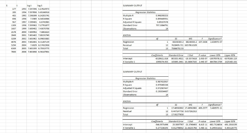
4. Repeat above procedure to determine the quadratic, cubic, logarithmic, and exponential functions of the best fit. Graph each function you obtained on the scatter diagram.

5. Select the regression model that you think best fits the data for sales and make a case for why you have chosen this model. 6. Based on the models you choose above, estimate the annual sales for 2008 and 2010. Compare your estimated value from the model to the exact sales in 2008 and 2010 (google to find the exact sales data). Also predict the sales for 2015 and 2020.

7. Using your model, find the table for rate of change of annual sales from 1993 to 2006.

8. Using your model, predict the total sales of the company from 1993 to 2020 in billion of dollars.

1-2:

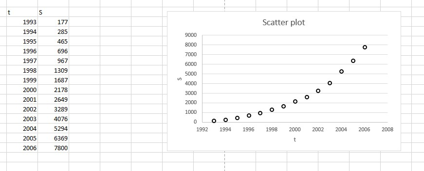From the shape of the data it is observed that S increases exponentially with t.

3.

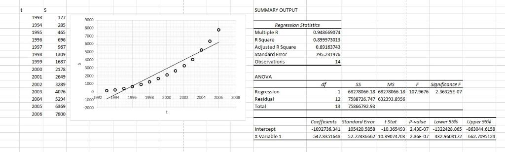
No. 90% of total variation of S is explained by this regression line.

4.

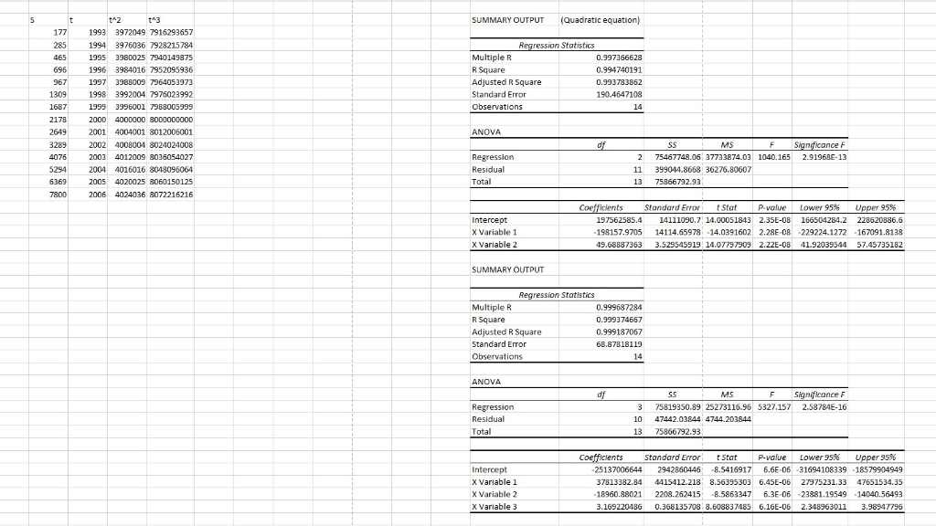
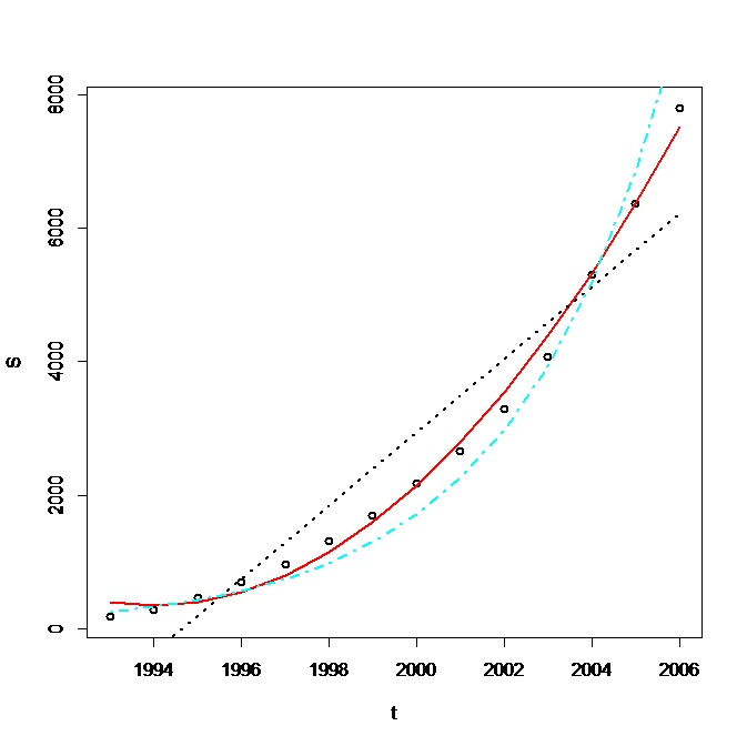
From the plot it is observed quadratic model gives best fit (see red line).

5.

Here black line is for logarithic and sky blue indicates exponential whereas cubic equation does not fit here.

Scatter plot 1992 1994 1996 1998 2000 2002 2004 2006 2008 -1092736.341 547.8352t S = 197562585.4-198 157.9705t + 49.68887363t2 with R2-0.9947 S25137006644+37813382.84t-18960.8802t2 +3.1692t3wit R0.9994 t 2 t03 SUMMARY OUTPUT(Quadratic equation) 1993 3972049 7916293657 1994 3976036 7928215784 1995 3980025 7940149875 1996 3984016 7952095936 1997 3988009 7964053973 1998 3992004 7976023992 1999 3996001 7988005995 2000 4000000 8000000000 2001 4004001 8012006001 2002 4008001 8024024008 2003 4012009 8036054027 2004 4016016 8048096064 2005 4020025 8060150125 2006 4024036 8072216216 ression Stotistics Multiple R R Square Adjusted R Square Standard Error Observations 0.997366628 0.994740191 0.993783862 190.4647108 ANOVA Significonce F MS 2 75467748.06 37733874.03 1040.165 2.91968E-13 Residual Total 11 399014.8668 36276.80607 13 75866792.93 Standard Error tStat P-value Lower 95% U , 95% 197562585.4 14111090.7 14.00051843 2.35E-08 16504284.2 228520886.6 198157.9705 14114.65978 14.03916022.28E 082292241272 167091.8138 49.68887363 3.529545919 14.07791909 2.22E-08 41.92039544 57.45735182 X Variable 1 X Variable 2 SUMMARY OUTPUT ression Stotistics Multiple R R Square Adjusted R Square Standard Error Observations 0.999687284 0.999374667 0.999187067 68.87818119 ANOVA F Significance F Regression 3 75819350.89 25273116.96 5327.157 2.58784E-16 10 47442.03844 4744 203844 13 75866792.93 Total Standard Error Lower 95% 95% Coe Stat P-value U 25137006644 2942860446 8.5416917 6.6E-06-31694108339 18579904949 37813382.84 4415412 218 8.56395303 6.45E-06 27975231.33 47651534.35 18960.88021 2208.262415 8.5863347 6.3E-06 23881.19549 14040.56493 3.169220486 0.368135708 8.608837485 6.16E-06 2.348963011 3.98547796 X Variable 1 X Variable 2 X Variable 3 =-8320621.818+ 1095074355 log t uith R2-0.8994 log S--546.9571+0.2772t Or. 546.9571 e0.2772t with R2=0.9751 Scatter plot 1992 1994 1996 1998 2000 2002 2004 2006 2008 -1092736.341 547.8352t S = 197562585.4-198 157.9705t + 49.68887363t2 with R2-0.9947 S25137006644+37813382.84t-18960.8802t2 +3.1692t3wit R0.9994 t 2 t03 SUMMARY OUTPUT(Quadratic equation) 1993 3972049 7916293657 1994 3976036 7928215784 1995 3980025 7940149875 1996 3984016 7952095936 1997 3988009 7964053973 1998 3992004 7976023992 1999 3996001 7988005995 2000 4000000 8000000000 2001 4004001 8012006001 2002 4008001 8024024008 2003 4012009 8036054027 2004 4016016 8048096064 2005 4020025 8060150125 2006 4024036 8072216216 ression Stotistics Multiple R R Square Adjusted R Square Standard Error Observations 0.997366628 0.994740191 0.993783862 190.4647108 ANOVA Significonce F MS 2 75467748.06 37733874.03 1040.165 2.91968E-13 Residual Total 11 399014.8668 36276.80607 13 75866792.93 Standard Error tStat P-value Lower 95% U , 95% 197562585.4 14111090.7 14.00051843 2.35E-08 16504284.2 228520886.6 198157.9705 14114.65978 14.03916022.28E 082292241272 167091.8138 49.68887363 3.529545919 14.07791909 2.22E-08 41.92039544 57.45735182 X Variable 1 X Variable 2 SUMMARY OUTPUT ression Stotistics Multiple R R Square Adjusted R Square Standard Error Observations 0.999687284 0.999374667 0.999187067 68.87818119 ANOVA F Significance F Regression 3 75819350.89 25273116.96 5327.157 2.58784E-16 10 47442.03844 4744 203844 13 75866792.93 Total Standard Error Lower 95% 95% Coe Stat P-value U 25137006644 2942860446 8.5416917 6.6E-06-31694108339 18579904949 37813382.84 4415412 218 8.56395303 6.45E-06 27975231.33 47651534.35 18960.88021 2208.262415 8.5863347 6.3E-06 23881.19549 14040.56493 3.169220486 0.368135708 8.608837485 6.16E-06 2.348963011 3.98547796 X Variable 1 X Variable 2 X Variable 3 =-8320621.818+ 1095074355 log t uith R2-0.8994 log S--546.9571+0.2772t Or. 546.9571 e0.2772t with R2=0.9751