this python program give me three plots, can I get a modified version where it prints a table of the data points for the plots?

import numpy as np

import matplotlib.pyplot as plt

# Constants

gamma $=1\mathrm{.}4$ # Specific heat ratio for air

CFL $=0\mathrm{.}5$ # $($Courant$-$Friedrichs$-$Lewy$)$

# Function to initialize grid and initial conditions

def initialize$\_$grid$($nx$,$ xmax, rho$\_$l$,$ u$\_$l$,$ p$\_$l$,$ rho$\_$r$,$ u$\_$r$,$ p$\_$r$)$:

dx $=$ xmax $/($nx $-1)$

x $=$ np$.$linspace$(0,$ xmax, nx$)$

rho $=$ np$.$zeros$($nx$)$

u $=$ np$.$zeros$($nx$)$

p $=$ np$.$zeros$($nx$)$

# Initial conditions

rho$[$x $$ xmax $/2]=$ rho$\_$l

rho$[$x $>=$ xmax $/2]=$ rho$\_$r

u$[$x $$ xmax $/2]=$ u$\_$l

u$[$x $>=$ xmax $/2]=$ u$\_$r

p$[$x $$ xmax $/2]=$ p$\_$l

p$[$x $>=$ xmax $/2]=$ p$\_$r

return x$,$ rho, u$,$ p$,$ dx

# Function to compute time step based on CFL condition

def compute$\_$dt$($dx$,$ u$)$:

dt $=$ CFL $*$ dx $/$ np$.$max$($np$.$abs$($u$)+$ np$.$sqrt$($gamma $*$ p $/$ rho$))$

return dt

# Function to update solution using Lax$-$Friedrichs scheme

def lax$\_$friedrichs$\_$step$($rho$,$ u$,$ p$,$ dt$,$ dx$)$:

rho$\_$n $=$ np$.$copy$($rho$)$

u$\_$n $=$ np$.$copy$($u$)$

p$\_$n $=$ np$.$copy$($p$)$

# Fluxes

F$\_$rho $=$ rho $*$ u

F$\_$u $=$ rho $*$ u $**2+$ p

F$\_$p $=($gamma $*$ p$)/($gamma $-1)*$ u $+0\mathrm{.}5*$ rho $*$ u $**3$

# Update solution

rho$\_$n$[1$:$-1]=0\mathrm{.}5*($rho$[$:$-2]+$ rho$[2$:$])-$ dt $/(2*$ dx$)*($F$\_$rho$[2$:$]-$ F$\_$rho$[$:$-2])$

u$\_$n$[1$:$-1]=0\mathrm{.}5*($u$[$:$-2]+$ u$[2$:$])-$ dt $/(2*$ dx$)*($F$\_$u$[2$:$]-$ F$\_$u$[$:$-2])$

p$\_$n$[1$:$-1]=0\mathrm{.}5*($p$[$:$-2]+$ p$[2$:$])-$ dt $/(2*$ dx$)*($F$\_$p$[2$:$]-$ F$\_$p$[$:$-2])$

return rho$\_$n$,$ u$\_$n$,$ p$\_$n

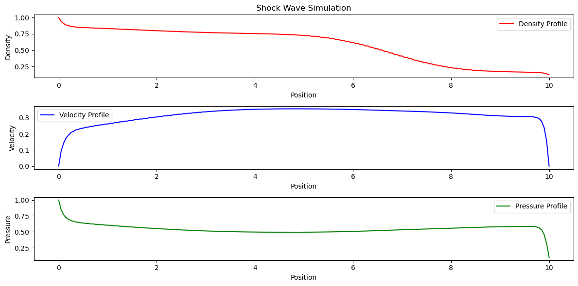
# Function to plot results

def plot$\_$results$($x$,$ rho, u$,$ p$,$ title$)$:

plt$.$figure$($figsize$=(12,6))$

plt$.$subplot$(3,1,1)$

plt$.$plot$($x$,$ rho, $\text{'}$r$-\text{'},$ label$=$'Density Profile'$)$ #$\text{'}$r$-$'stand for the wave color red

plt$.$xlabel$(\text{'}$Position$\text{'})$

plt$.$ylabel$(\text{'}$Density$\text{'})$

plt$.$title$($title$)$

plt$.$legend$()$

plt$.$subplot$(3,1,2)$

plt$.$plot$($x$,$ u$,\text{'}$b$-\text{'},$ label$=$'Velocity Profile'$)$ #$\text{'}$b$-$'stand for the wave color blue

plt$.$xlabel$(\text{'}$Position$\text{'})$

plt$.$ylabel$(\text{'}$Velocity$\text{'})$

plt$.$legend$()$

plt$.$subplot$(3,1,3)$

plt$.$plot$($x$,$ p$,\text{'}$g$-\text{'},$ label$=$'Pressure Profile'$)$ #$\text{'}$g$-$'stand for the wave color green

plt$.$xlabel$(\text{'}$Position$\text{'})$

plt$.$ylabel$(\text{'}$Pressure$\text{'})$

plt$.$legend$()$

plt$.$tight$\_$layout$()$

plt$.$show$()$

# Parameters of the plots

nx $=201$ # Number of grid points

xmax $=10\mathrm{.}0$ # Maximum x value

rho$\_$l $=1\mathrm{.}0$ # Left density

u$\_$l $=0\mathrm{.}0$ # Left velocity

p$\_$l $=1\mathrm{.}0$ # Left pressure

rho$\_$r $=0\mathrm{.}125$ # Right density

u$\_$r $=0\mathrm{.}0$ # Right velocity

p$\_$r $=0\mathrm{.}1$ # Right pressure

T $=5\mathrm{.}0$ # Total simulation time

# Initialize grid and initial conditions

x$,$ rho, u$,$ p$,$ dx $=$ initialize$\_$grid$($nx$,$ xmax, rho$\_$l$,$ u$\_$l$,$ p$\_$l$,$ rho$\_$r$,$ u$\_$r$,$ p$\_$r$)$

# Main loop

t $=0\mathrm{.}0$

while t $$ T:

dt $=$ compute$\_$dt$($dx$,$ u$)$

rho, u$,$ p $=$ lax$\_$friedrichs$\_$step$($rho$,$ u$,$ p$,$ dt$,$ dx$)$

t $+=$ dt

# Plot results

plot$\_$results$($x$,$ rho, u$,$ p$,$ 'Shock Wave Simulation'$)$

Output:

Shock Wave Simulation