thumbs up if solved coreectly. Ty

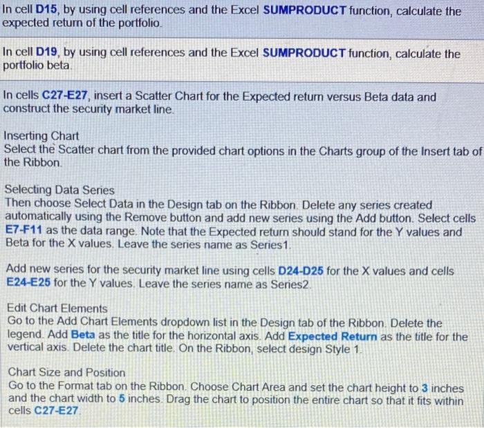
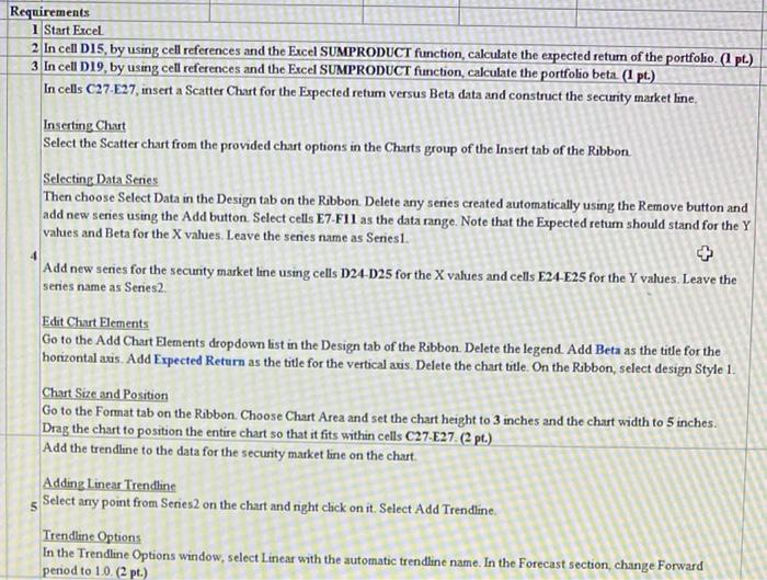
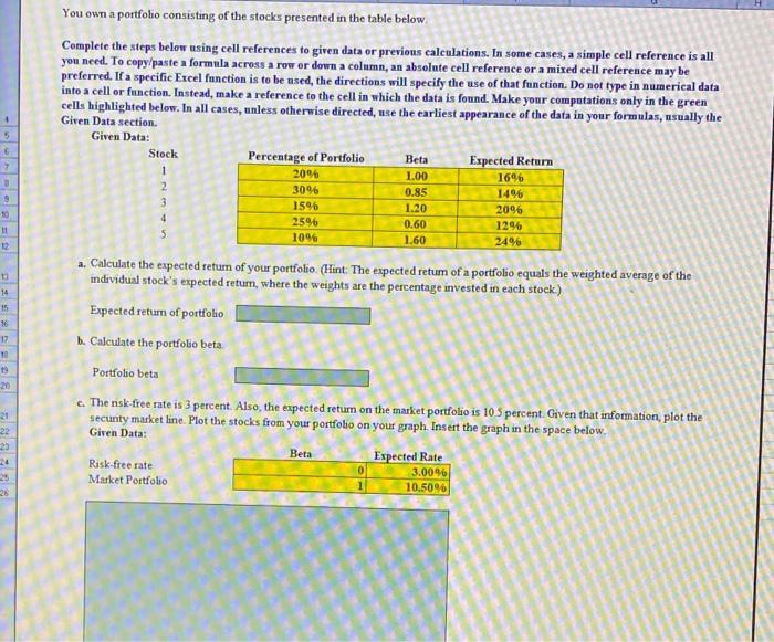
In cell D15, by using cell references and the Excel SUMPRODUCT function, calculate the expected return of the portfolio. In cell D19, by using cell references and the Excel SUMPRODUCT function, calculate the portfolio beta In cells C27-E27, insert a Scatter Chart for the Expected return versus Beta data and construct the security market line. Inserting Chart Select the Scatter chart from the provided chart options in the Charts group of the Insert tab of the Ribbon Selecting Data Series Then choose Select Data in the Design tab on the Ribbon Delete any series created automatically using the Remove button and add new series using the Add button. Select cells E7-F11 as the data range. Note that the Expected return should stand for the Y values and Beta for the X values. Leave the series name as Series1 Add new series for the security market line using cells D24-D25 for the X values and cells E24-E25 for the Y values. Leave the series name as Series2 Edit Chart Elements Go to the Add Chart Elements dropdown list in the Design tab of the Ribbon. Delete the legend. Add Beta as the title for the horizontal axis. Add Expected Return as the title for the vertical axis Delete the chart title. On the Ribbon, select design Style 1 Chart Size and Position Go to the Format tab on the Ribbon. Choose Chart Area and set the chart height to 3 inches and the chart width to 5 inches Drag the chart to position the entire chart so that it fits within cells C27-E27 Requirements 1 Start Excel 2 In cell D15, by using cell references and the Excel SUMPRODUCT function calculate the expected retum of the portfolio.pl.) 3 In cell D19, by using cell references and the Excel SUMPRODUCT function, calculate the portfolio beta (1 pt.) In cells C27-E27, insert a Scatter Chart for the Expected return versus Beta data and construct the security market line Inserting Chart Select the Scatter chart from the provided chart options in the Charts group of the Insert tab of the Ribbon Selecting Data Senes Then choose Select Data in the Design tab on the Ribbon. Delete any series created automatically using the Remove button and add new series using the Add button. Select cells E7-F11 as the data range. Note that the Expected retum should stand for the Y values and Beta for the X values. Leave the series name as Seniesl. Add new series for the security market line using cells 024-D25 for the X values and cells E24-E25 for the Y values. Leave the series name as Series2 4 Edit Chart Elements Go to the Add Chart Elements dropdown list in the Design tab of the Ribbon. Delete the legend. Add Beta as the title for the horizontal axis. Add Expected Return as the title for the vertical avis. Delete the chart title. On the Ribbon, select design Style 1 Chart Site and Position Go to the Format tab on the Ribbon. Choose Chart Area and set the chart height to 3 inches and the chart width to 5 inches. Drag the chart to position the entire chart so that it fits within cells C27-E27Cpt.) Add the trendline to the data for the security market line on the chart. Adding Linear Trendline s Select any point from Series2 on the chart and night click on it. Select Add Trendline. Trendline Options In the Trendline Options window, select Linear with the automatic trendline name. In the Forecast section change Forward period to 1.0. (2 pt.) You own a portfolio consisting of the stocks presented in the table below. Complete the steps below using cell references to given data or previous calculations. In some cases, a simple cell reference is all you need. To copy/paste a formula across a row or down a column, an absolute cell reference or a mixed cell reference may be preferred. If a specific Excel function is to be used, the directions will specify the use of that function. Do not type in numerical data into a cell or function. Instead, make a reference to the cell in which the data is found. Make your computations only in the green cells highlighted below. In all cases, unless otherwise directed, use the earliest appearance of the data in your formulas, usually the Given Data section. Given Data: Percentage of Portfolio Expected Return 16% 3096 5 2096 Stock 1 2 3 4 9 10 11 2 Beta 1.00 0.85 1.20 0.60 1.60 1596 25 1096 1496 2096 12% 2496 14 15 16 17 10 a. Calculate the expected return of your portfolio. (Hint: The expected retum of a portfolio equals the weighted average of the individual stock's expected return, where the weights are the percentage invested in each stock) Expected return of portfolio b. Calculate the portfolio beta Portfolio beta c. The risk-free rate is 3 percent. Also, the expected return on the market portfolio is 105 percent. Given that information, plot the secunty market line. Plot the stocks from your portfolio on your graph. Insert the graph in the space below. Given Data: Beta Expected Rate Risk free rate 3.0096 Market Portfolio 20 21 22 25 26 10.5096