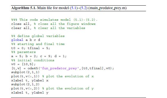
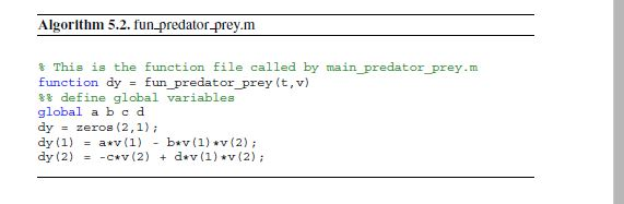
To write MATLAB codes for the following problems, we can refer to Algorithms 5.1 and 5.2 in Chapter 5. Problem 6.6. Consider the dynamical system (6.7)(6.8) with u = 1, n = 1,2, r2 = 1,4, K = 3, and x(0) = 2, y(0) = 1, so that x(t) > y(t) fort small. Simulate the system for t> 0 until you arrive at time T such that y(T) = x(T). Problem 6.10. Implement the backward Euler method for y=-y2 +t, y(0) = 1, Ostsi. Use h = 0.01, 0.005 0.001. (Hint: you have to solve a quadratic equation at each time step.] Algorithm 5.1. Main file for model (5.1) (5.2) (main_predator_prey.m) 888 This code simulates model (5.1) - (5.2). close all, close all the figure windows clear all, clear all the variables 8% define global variables global a b c d 88 starting and final time t0 = 0; tfinal = 5; 8% paramters a = 5; b = 2; c = 9; d = 1; %% initial conditions v0 = [10,5); [t, v] = ode45 ('fun_predator prey', [t0,tfinal],vo); subplot (2,1,1) plot(t,v(:,1)) $ plot the evolution of x xlabel t, ylabel x subplot (2,1,2) plot(t,v(:,2)) plot the evolution of y xlabel t, ylabel y Algorithm 5.2. fun predator prey.m $ This is the function file called by main predator prey.m function dy = fun_predator_prey (t,v) 8% define global variables global a bed dy = zeros (2,1); dy (1) = a*v (1) - buv(1) *v (2); dy (2) = -cwv(2) + dev(1) *v (2)