using r software

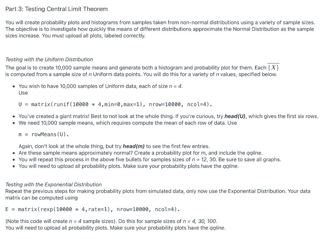
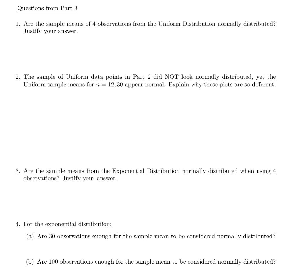
Part 3: Testing Central Limit Theorem You will create probability plots and histograms from samples taken from non-normal distributions using a variety of sample sizes. The objective is to investigate how quickly the means of different distributions approximate the Normal Distribution as the sample sizes increase. You must upload all plots, labeled correctly. Testing with the Uniform Distribution The goal is to create 10,000 sample means and generate both a histogram and probability plot for them. Each {X} is computed from a sample size of n Uniform data points. You will do this for a variety of n values, specified below. . You wish to have 10,000 samples of Uniform data, each of size n = 4. Use U = matrix(runif (10000 * 4, min=0,max=1), nrow=10000, ncol=4). You've created a giant matrix! Best to not look at the whole thing. If you're curious, try head(U), which gives the first six rows. We need 10,000 sample means, which requires compute the mean of each row of data. Use m = rowMeans (U). Again, don't look at the whole thing, but try head(m) to see the first few entries. Are these sample means approximately normal? Create a probability plot for m, and include the qoline. You will repeat this process in the above five bullets for samples sizes of n = 12, 30. Be sure to save all graphs. You will need to upload all probability plots. Make sure your probability plots have the qqline. Testing with the Exponential Distribution Repeat the previous steps for making probability plots from simulated data, only now use the Exponential Distribution. Your data matrix can be computed using E = matrix(rexp(10000 * 4, rate=1), nrow=10000, ncol=4). (Note this code will create n = 4 sample sizes). Do this for sample sizes of n = 4, 30, 100. You will need to upload all probability plots. Make sure your probability plots have the qqline. Questions from Part 3 1. Are the sample means of 4 observations from the Uniform Distribution normally distributed? Justify your answer. 2. The sample of Uniform data points in Part 2 did NOT look normally distributed, yet the Uniform sample means for n = 12,30 appear normal. Explain why these plots are so different. 3. Are the sample means from the Exponential Distribution normally distributed when using 4 observations? Justify your answer. 4. For the exponential distribution: (a) Are 30 observations enough for the sample mean to be considered normally distributed? (b) Are 100 observations enough for the sample mean to be considered normally distributed? Part 3: Testing Central Limit Theorem You will create probability plots and histograms from samples taken from non-normal distributions using a variety of sample sizes. The objective is to investigate how quickly the means of different distributions approximate the Normal Distribution as the sample sizes increase. You must upload all plots, labeled correctly. Testing with the Uniform Distribution The goal is to create 10,000 sample means and generate both a histogram and probability plot for them. Each {X} is computed from a sample size of n Uniform data points. You will do this for a variety of n values, specified below. . You wish to have 10,000 samples of Uniform data, each of size n = 4. Use U = matrix(runif (10000 * 4, min=0,max=1), nrow=10000, ncol=4). You've created a giant matrix! Best to not look at the whole thing. If you're curious, try head(U), which gives the first six rows. We need 10,000 sample means, which requires compute the mean of each row of data. Use m = rowMeans (U). Again, don't look at the whole thing, but try head(m) to see the first few entries. Are these sample means approximately normal? Create a probability plot for m, and include the qoline. You will repeat this process in the above five bullets for samples sizes of n = 12, 30. Be sure to save all graphs. You will need to upload all probability plots. Make sure your probability plots have the qqline. Testing with the Exponential Distribution Repeat the previous steps for making probability plots from simulated data, only now use the Exponential Distribution. Your data matrix can be computed using E = matrix(rexp(10000 * 4, rate=1), nrow=10000, ncol=4). (Note this code will create n = 4 sample sizes). Do this for sample sizes of n = 4, 30, 100. You will need to upload all probability plots. Make sure your probability plots have the qqline. Questions from Part 3 1. Are the sample means of 4 observations from the Uniform Distribution normally distributed? Justify your answer. 2. The sample of Uniform data points in Part 2 did NOT look normally distributed, yet the Uniform sample means for n = 12,30 appear normal. Explain why these plots are so different. 3. Are the sample means from the Exponential Distribution normally distributed when using 4 observations? Justify your answer. 4. For the exponential distribution: (a) Are 30 observations enough for the sample mean to be considered normally distributed? (b) Are 100 observations enough for the sample mean to be considered normally distributed