We have a theoretical result that guarantees a certain quality of the approximation of a sufficiently smooth function by an interpolation polynomial. In this task, you will learn to interpret this result properly, and you will see that applying a numerical method to a seemingly nice problem without checking the theoretical background is potentially dangerous

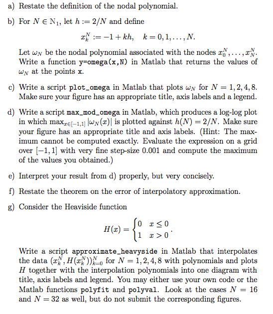
a) Restate the definition of the nodal polynomial b) For N N 1, let h := 2/N and define 1kh, k 0,1,... ,N. Let wv be the nodal polynomial associated with the nodes ^y,... , TN Write a function y-omega(x,N) in Matlab that returns the values of wN at the points x. c) Write a script plot-omega in Matlab that plots uw for N 1,2,4,8 Make sure your figure has an appropriate title, axis labels and a legend d) Write a script max_mod_omega in Matlab, which produces a log-log plot in which maxrl-1.1 lwN(x) is plotted against h(N) - 2/N. Make sure your figure has an appropriate title and axis labels. (Hint: The max- imum cannot be computed exactly. Evaluate the expression on a grid over [-1,1] with very fine step-size 0.001 and compute the maximum of the values you obtained.) e) Interpret your result from d) properly, but very concisely. f) Restate the theorem on the error of interpolatory approximation. g) Consider the Heaviside function H (z) = Write a script approximate_heavyside in Matlab that interpolates the data (zr, H(2))0 for N = 1, 2, 4,8 with polynomials and plots H together with the interpolation polynomials into one diagram with title, axis labels and legend. You may either use your own code or the Matlab functions polyfit and polyval. Look at the cases N 16 and N - 32 as well, but do not submit the corresponding figures a) Restate the definition of the nodal polynomial b) For N N 1, let h := 2/N and define 1kh, k 0,1,... ,N. Let wv be the nodal polynomial associated with the nodes ^y,... , TN Write a function y-omega(x,N) in Matlab that returns the values of wN at the points x. c) Write a script plot-omega in Matlab that plots uw for N 1,2,4,8 Make sure your figure has an appropriate title, axis labels and a legend d) Write a script max_mod_omega in Matlab, which produces a log-log plot in which maxrl-1.1 lwN(x) is plotted against h(N) - 2/N. Make sure your figure has an appropriate title and axis labels. (Hint: The max- imum cannot be computed exactly. Evaluate the expression on a grid over [-1,1] with very fine step-size 0.001 and compute the maximum of the values you obtained.) e) Interpret your result from d) properly, but very concisely. f) Restate the theorem on the error of interpolatory approximation. g) Consider the Heaviside function H (z) = Write a script approximate_heavyside in Matlab that interpolates the data (zr, H(2))0 for N = 1, 2, 4,8 with polynomials and plots H together with the interpolation polynomials into one diagram with title, axis labels and legend. You may either use your own code or the Matlab functions polyfit and polyval. Look at the cases N 16 and N - 32 as well, but do not submit the corresponding figures