Reconsider the data in Exercise 14.4. Define a new set of transformed variables as the first difference of the original variables, \(y_{t}^{\prime}=y_{t}-y_{t-1}\) and \(x_{t}^{\prime}=x_{t}-x_{t-1}\). Regress \(y_{t}^{\prime}\) on \(x_{t}^{\prime}\) through the origin. Compare the estimate of the slope from this first-difference approach with the estimate obtained from the iterative method in Exercise 14.4.

Data From Exercises 14.4

The data in the following table gives the monthly sales for a cosmetics manufacturer (yt)$\left({\mathrm{????}}_{\mathrm{????}}\right)$ and the corresponding monthly sales for the entire industry (xt)$\left({\mathrm{????}}_{\mathrm{????}}\right)$. The units of both variables are millions of dollars.
a. Build a simple linear regression model relating company sales to industry sales. Plot the residuals against time. Is there any indication of autocorrelation?
b. Use the Durbin-Watson test to determine if there is positive autocorrelation in the errors. What are your conclusions?
c. Use one iteration of the Cochrane-Orcutt procedure to estimate the model parameters. Compare the standard error of these regression coefficients with the standard error of the least-squares estimates.
d. Test for positive autocorrelation following the first iteration. Has the procedure been successful?

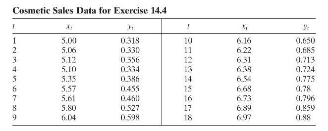
Cosmetic Sales Data for Exercise 14.4 t X t X 1 5.00 0.318 10 6.16 0.650 2 5.06 0.330 11 6.22 0.685 3 5.12 0.356 12 6.31 0.713 456789 5.10 0.334 13 6.38 0.724 5.35 0.386 14 6.54 0.775 5.57 0.455 15 6.68 0.78 5.61 0.460 16 6.73 0.796 5.80 0.527 17 6.89 0.859 6.04 0.598 18 6.97 0.88