New Semester Started Get 50% OFF Study Help! --h --m --s Claim Now

Question Answers

Textbooks

Find textbooks, questions and answers

Oops, something went wrong!

Change your search query and then try again

Result Not Found

Books FREE
Study Help
Tutors
AI Study Planner NEW
Sell Books

Search
Sign In
Register

study help
mathematics
calculus

Modeling the Dynamics of Life Calculus and Probability for Life Scientists 3rd edition Frederick R. Adler - Solutions

Graph a rate-of-change function that has a slope of 0 at the equilibrium but the equilibrium is unstable. What is the sign of the second derivative at the equilibrium? What is the sign of the third derivative at the equilibrium? As with discrete-time dynamical systems, equilibria can act strange
Try to draw a phase-line diagram with two stable equilibria in a row. Use the Intermediate Value Theorem to sketch a proof of why this is impossible. The fact that the rate-of-change function is continuous means that many behaviors are impossible for an autonomous differential equation.
Why is it impossible for a solution of an autonomous differential equation to oscillate? The fact that the rate-of-change function is continuous means that many behaviors are impossible for an autonomous differential equation.
Consider the equationfor both positive and negative values of x. Find the equilibria as functions of a for values of a between -1 and 1. Draw a bifurcation diagram and describe in words what happens at a = 0. The change that occurs at a = 0 is called a transcritical bifurcation.When parameter
Consider the equationfor both positive and negative values of x. Find the equilibria as functions of a for values of a between -1 and 1. Draw a bifurcation diagram and describe in words what happens at a = 0. The change that occurs at a = 0 is called a saddle-node bifurcation.When parameter values
Consider the equationfor both positive and negative values of x. Find the equilibria as functions of a for values of a between -1 and 1. Draw a bifurcation diagram and describe in words what happens at a = 0. The change that occurs at a = 0 is called a pitchfork bifurcation.When parameter values
From the following graphs of the rate of change as a function of the state variable, identify stable and unstable equilibria by checking whether the rate of change is an increasing or decreasing function of the state variable.
Consider the equationfor both positive and negative values of x. Find the equilibria as functions of a for values of a between -1 and 1. Draw a bifurcation diagram and describe in words what happens at a = 0. The change that occurs at a = 0 is a slightly different type of pitchfork bifurcation
Use the stability theorem to check the phase-line diagrams for the following models of bacterial population growth.1. The model in Section 5.1, Exercise 27 and Section 5.2 Exercise 21.2. The model in Section 5.1, Exercise 28 and Section 5.2, Exercise 22.3. The model in Section 5.1, Exercise 29 and
Use the stability theorem to check the phase-line diagrams for the following models of bacterial population growth.1. The model in Section 5.1, Exercise 37 and Section 5.2, Exercise 27.2. The model in Section 5.1, Exercise 38 and Section 5.2, Exercise 28.
A reaction-diffusion equation describes how chemical concentration changes due to two factors simultaneously, reaction and movement. A simple model has the formThe first term describes diffusion, and the second term R(C) is the reaction, which could have a positive or negative sign (depending on
A reaction-diffusion equation describes how chemical concentration changes due to two factors simultaneously, reaction and movement. A simple model has the formThe first term describes diffusion, and the second term R(C) is the reaction, which could have a positive or negative sign (depending on
A reaction-diffusion equation describes how chemical concentration changes due to two factors simultaneously, reaction and movement. A simple model has the formThe first term describes diffusion, and the second term R(C) is the reaction, which could have a positive or negative sign (depending on
Use the stability theorem to evaluate the stability of the equilibria of the following autonomous differential equations.Compare your results with the phase line in Section 5.2, Exercise 15.
A reaction-diffusion equation describes how chemical concentration changes due to two factors simultaneously, reaction and movement. A simple model has the formThe first term describes diffusion, and the second term R(C) is the reaction, which could have a positive or negative sign (depending on
Apply the stability theorem for autonomous differential equations to the following equations. Show that your results match what you found in your phase-line diagrams, and give a biological interpretation.The equation
Apply the stability theorem for autonomous differential equations to the following equations. Show that your results match what you found in your phase-line diagrams, and give a biological interpretation.The equation
Apply the stability theorem for autonomous differential equations to the following equations. Show that your results match what you found in your phase-line diagrams, and give a biological interpretation. The equation dv/dt = a - Dv2 with a = 9.8m/s2 and D = 0.0032 per meter.
Apply the stability theorem for autonomous differential equations to the following equations. Show that your results match what you found in your phase-line diagrams, and give a biological interpretation. The equation dv/dt = a - Dv2 with a = 9.8m/s2 and D = 0.00048 per meter.
Apply the stability theorem for autonomous differential equations to the following equations. Show that your results match what you found in your phase-line diagrams, and give a biological interpretation. The equation dy/dt = -c√y with c = 2.0√cm/s.
The equation from the previous problem but with water entering at a rate of 4.0 cm/s. Apply the stability theorem for autonomous differential equations to the following equations. Show that your results match what you found in your phase-line diagrams, and give a biological interpretation. Previous
Apply the stability theorem for autonomous differential equations to the following equations. Show that your results match what you found in your phase-line diagrams, and give a biological interpretation. The equation dS/dt = -S/1 + S
The equation from the previous problem but with substrate added at rate R = 0.5. Apply the stability theorem for autonomous differential equations to the following equations. Show that your results match what you found in your phase-line diagrams, and give a biological interpretation. Previous
Apply the stability theorem for autonomous differential equations to the following equations. Show that your results match what you found in your phase-line diagrams, and give a biological interpretation. The equation dV/dt = a1V2/3 - a2V.
Use the stability theorem to evaluate the stability of the equilibria of the following autonomous differential equations.Compare your results with the phase line in Section 5.2, Exercise 16.
Apply the stability theorem for autonomous differential equations to the following equations. Show that your results match what you found in your phase-line diagrams, and give a biological interpretation. The equation dV/dt = a1V2/3 - a2V3/4.
Consider the logistic differential equation (Section 5.1, Exercise 27) with harvesting proportional to population size, or db/dt = b(1 - b - h) where h represents the fraction harvested. Graph the equilibria as functions of h for values of h between 0 and 2, using a solid line when an equilibrium
Suppose μ = 1 in the basic disease model dI/dt = αI(1 - I) - μI. Graph the two equilibria as functions of α for values of a between 0 and 2, using a solid line when an equilibrium is stable and a dashed line when an equilibrium is unstable. Even though they do not make biological sense, include
Consider a version of the equation in Section 5.2, Exercise 29 that includes the parameter r,Graph the equilibria as functions of r for values of r between 0 and 3, using a solid line when an equilibrium is stable and a dashed line when an equilibrium is unstable. The algebra for checking stability
Consider a variant of the basic disease model given byGraph the equilibria as functions of Î± for values of Î± between 0 and 5, using a solid line when an equilibrium is stable and a dashed line when an equilibrium is unstable. The algebra for checking stability is messy, so it is only
Analyze the stability of the positive equilibrium in the model from Exercise 44 when α = 4, the point where the bifurcation occurs. Right at a bifurcation point, the stability theorem fails because the slope of the rate-of-change function at the equilibrium is exactly zero. In each of the
Analyze the stability of the disease model when α = μ = 1, the point where the bifurcation occurs in Exercise 42. Right at a bifurcation point, the stability theorem fails because the slope of the rate-of-change function at the equilibrium is exactly zero. In each of the following cases, check
Use the stability theorem to evaluate the stability of the equilibria of the following autonomous differential equations.Compare your results with the phase line in Section 5.2, Exercise 17.
Use the stability theorem to evaluate the stability of the equilibria of the following autonomous differential equations.Compare your results with the phase line in Section 5.2, Exercise 18.
Find the stability of the equilibria of the following autonomous differential equations that include parameters.Suppose that a > 0.
Use separation of variables to solve the following autonomous differential equations. Check your answers by differentiating.
Use separation of variables to solve the following pure-time differential equations. Check your answers by differentiating.
Find the solution of the differential equation db/dt = bp in the following cases. At what time does it approach infinity? Sketch a graph. p = 2 (as in the text) and b(0) = 100.
Find the solution of the differential equation db/dt = bp in the following cases. At what time does it approach infinity? Sketch a graph. p = 2 and b(0) = 0.1.
Find the solution of the differential equation db/dt = bp in the following cases. At what time does it approach infinity? Sketch a graph. p = 1.1 and b(0) = 100.
Find the solution of the differential equation db/dt = bp in the following cases. At what time does it approach infinity? Sketch a graph. p = 1.1 and b(0) = 0.1.
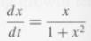
The autonomous differential equationwith x(0) = 1. This describes a population with per capita production that decreases like 1/1 + x.The following autonomous differential equations can be solved except for the step of finding x in terms of t. Use the steps to figure out how the solution behaves.a.
The autonomous differential equationwith x(0) = l. This describes a population with per capita production that decreases like 1/1 + x2. Describe in words how the solution differs from that in Exercise 15.The following autonomous differential equations can be solved except for the step of
Show that the solution comes out the same if N > K. Check the above results about the solution of the logistic equation from Example 5.4.7.
Differentiate to check that the solution given in Example 5.4.7 solves the differential equation. Check the above results about the solution of the logistic equation from Example 5.4.7.
Using the method used to find the solution derived for Newton's law of cooling, find the solution of the chemical diffusion equation dC/dt = β(Г - C) with the following parameter values and initial conditions. Find the concentration after 10 seconds. How long would it take for the concentration
Use separation of variables to solve the following autonomous differential equations. Check your answers by differentiating.
Using the method used to find the solution derived for Newton's law of cooling, find the solution of the chemical diffusion equation dC/dt = β(Г - C) with the following parameter values and initial conditions. Find the concentration after 10 seconds. How long would it take for the concentration
Suppose the initial condition is y(0) = 4. Find the solution with separation of variables and graph the result. What really happens at time t = 2? And what happens after this time? How does this differ from the solution of the equation dy/dt = -2y? Consider Torricelli's law of draining dy/dt =
Suppose the initial condition is y(0) = 16. Find the solution with separation of variables and graph the result. When does the solution reach 0? What would the depth be at this time if draining followed the equation dy/dt = -2y? Consider Torricelli's law of draining dy/dt = -2√y (Section 5.2,
Suppose a population is growing at constant rate λ, but that individuals are harvested at a rate of h, following the differential equation db/dt = λb - h. For each of the following values of λ and h, use separation of variables to find the solution, and compare graphs of the solution with those
Suppose a population is growing at constant rate λ, but that individuals are harvested at a rate of h, following the differential equation db/dt = λb - h. For each of the following values of λ and h, use separation of variables to find the solution, and compare graphs of the solution with those
Use separation of variables to solve for C in the following models describing chemical diffusion, and find the solution starting from the initial condition C = Г.1. The model in Section 5.1, Exercise 33.2. The model in Section 5.1, Exercise 34.
Separation of variables can help to solve some non autonomous differential equations. For example, suppose that the per capita production rate is λ(t), a function of time, so that db/dt =λ(t)b.
Use separation of variables to solve the following autonomous differential equations. Check your answers by differentiating.
Separation of variables can help to solve some non autonomous differential equations. For example, suppose that the per capita production rate is λ(t), a function of time, so that db/dt =λ(t)b. Discuss.
Separation of variables can help to solve some non autonomous differential equations. For example, suppose that the per capita production rate is λ(t), a function of time, so that db/dt =λ(t)b. Discuss in detail.
Separation of variables can help to solve some non autonomous differential equations. For example, suppose that the per capita production rate is λ(t), a function of time, so that db/dt =λ(t)b. Discuss briefly.
The model from Section 5.1, Exercise 29 with initial condition b(0) = 100.
The model from Section 5.1, Exercise 30 with initial condition b(0) = 10.000.
Find the solution of Equation 5.1.4 as a special case of the logistic equation and compare with the solution in Equation 5.1.6. Our model of selection (Equation 5.1.4) looks much like the logistic equation studied in Example 5.4.7, but can be extended to be frequency-dependent when the fitness of
Suppose that μ = 2 - 2p and λ = 1. Find the equilibria and their stability. What method would you use to try to find the solution after separating variables? Our model of selection (Equation 5.1.4) looks much like the logistic equation studied in Example 5.4.7, but can be extended to be
Create the new variable y = et H and find a differential equation for y. There are many important differential equations for which separation of variables fails, but which can be solved with other techniques. An important category involves Newton's law of cooling when the ambient temperature is
Identify the type of differential equation, and solve it with the initial condition H(0) = 0. There are many important differential equations for which separation of variables fails, but which can be solved with other techniques. An important category involves Newton's law of cooling when the
Graph your solution and the ambient temperature when β is small, say β = 0.1. Describe the result. There are many important differential equations for which separation of variables fails, but which can be solved with other techniques. An important category involves Newton's law of cooling when
Use separation of variables to solve the following autonomous differential equations. Check your answers by differentiating.
Graph your solution and the ambient temperature when β is large, say β = 1.0. Why are the two curves so much farther apart? There are many important differential equations for which separation of variables fails, but which can be solved with other techniques. An important category involves
Use separation of variables to solve the following autonomous differential equations. Check your answers by differentiating.
Use separation of variables to solve the following autonomous differential equations. Check your answers by differentiating.
Use separation of variables to solve the following pure-time differential equations. Check your answers by differentiating.
Use separation of variables to solve the following pure-time differential equations. Check your answers by differentiating.
Use separation of variables to solve the following pure-time differential equations. Check your answers by differentiating.
Consider the following special cases of the predator-prey equationsWrite the differential equations and say what they mean.ˆˆ = Î· = 0.
Start from a = 250 and b = 500. Take four steps, with a step length of Î”t = 0.05. How do your results compare with those in Exercise 8?Apply Euler's method to the competition equationsstarting from the given initial conditions. Assume that Î¼ = 2.0, Î» = 2.0, Ka = 1000, and Kb = 500.
Suppose Î± = 0.3 and Î±2 = 0.1. Start from H = 60 and A = 20. Take two steps, with a step length of Î”t = 0.1.Apply Euler's method to Newton's law of coolingwith the given parameter values and starting from the given initial conditions.
Suppose Î± = 0.3 and Î±2 = 0.1. Start from H = 0 and A = 20. Take two steps, with a step length of Î”t = 0.1.Apply Euler's method to Newton's law of coolingwith the given parameter values and starting from the given initial conditions.
Supposes Î± = 3.0 and Î±2 = 1.0. Start from H = 60 and A = 20. Take two steps, with a step length of Î”t = 0.25. Do the results look reasonable?Apply Euler's method to Newton's law of coolingwith the given parameter values and starting from the given initial conditions.
Suppose Î± = 3.0 and Î±2 = l.0. Start from H = 0 and A = 20. Take two steps, with a step length of Î”t = 0.5. Do the results look reasonable?Apply Euler's method to Newton's law of coolingwith the given parameter values and starting from the given initial conditions.
Write the velocity v in terms of the derivative of the position x, and the acceleration in terms of the derivative of the velocity v. Use the spring equation to write the derivative of the velocity in terms of the position x. Write the spring equation as a pair of equations for position and
Friction also creates acceleration proportional to the negative of the velocity (see Section 2.10, Exercise 39). A simple case obeys the equationWrite this as a pair of coupled differential equations for x and v.The spring equation or simple harmonic oscillatorstudied in Subsection 2.10.3 describes
We know that one solution of the basic spring equation in Exercise 15 is x(t) = cos(t). Find v(t) and check that the solution matches the system of equations. What are the initial position and velocity?The spring equation or simple harmonic oscillatorstudied in Subsection 2.10.3 describes how
One solution of the spring equation with friction in Exercise 16 is x(t) = e–t cos(t). Find v(t) and check that the solution matches the system of equations. What are the initial position and velocity?The spring equation or simple harmonic oscillatorstudied in Subsection 2.10.3 describes how
Use Euler's method with Î”t = 0.2 for five steps to estimate x(1) and v(1) for the model in Exercise 15 with initial position x(0) = 1 and initial velocity v(0) = 0. Compare with the results in Exercise 17.The spring equation or simple harmonic oscillatorstudied in Subsection 2.10.3 describes
Consider the following special cases of the predator-prey equationsWrite the differential equations and say what they mean.Î´ = 0.
Use Euler's method with Î”t = 0.2 for five steps to estimate x(1) and v(1) for the model in Exercise 16 with initial position x(0) = 1 and initial velocity v(0) = -1. Compare with the results in Exercise 18.The spring equation or simple harmonic oscillatorstudied in Subsection 2.10.3 describes
Non autonomous differential equations can be written as a system of coupled autonomous differential equations by writing a separate differential equation for the variable t.1. Write the differential equation dF/dt = F2 + kt (from Section 5.1, Exercise 1) as two equations for F and t.2. Write the
Per capita growth of prey = 1.0 - 0.05p Per capita growth of predators = -1.0 + 0.02b. Consider the above type of predator-prey interactions. Graph the per capita rates of change and write the associated system of autonomous differential equations.
Per capita growth of prey = 2.0 - 0.01p Per capita growth of predators = 1.0 + 0.01b. How does this differ from the basic predator-prey system (Equation 5.5.1)? Consider the above type of predator-prey interactions. Graph the per capita rates of change and write the associated system of autonomous
Per capita growth of prey = 2.0 - 0.0001p2 per capita growth of predators = -1.0 + 0.01b Consider the above type of predator-prey interactions. Graph the per capita rates of change and write the associated system of autonomous differential equations.
per capita growth of prey = 2.0 - 0.01p per capita growth of predators = -1.0 + 0.0001b2 Consider the above type of predator-prey interactions. Graph the per capita rates of change and write the associated system of autonomous differential equations.
Write systems of differential equations describing the above situation. Feel free to make up parameter values as needed.1. Two predators that must eat each other to survive.2. Two predators that must eat each other to survive, but with per capita production of each reduced by competition with its
Consider the following special cases of the predator-prey equationsWrite the differential equations and say what they mean.Î· = 0.
Suppose that the size of the first cell is 2.0 μL and the second is 5.0 μL.Follow these steps to derive the equations for chemical exchange between two adjacent cells of different size. Suppose the concentration in the first cell is designated by the variable C1, and the concentration in the
Suppose that the size of the first cell is 5.0 μL and the second is 12.0 μL.Follow these steps to derive the equations for chemical exchange between two adjacent cells of different size. Suppose the concentration in the first cell is designated by the variable C1, and the concentration in the
The size of the room is 10.0 times that of the object, but the specific heat of the room is 0.2 times that of the object (meaning that a small amount of heat can produce a large change in the temperature of the room). Write systems of autonomous differential equations describing the temperature of
The size of the room is 5.0 times that of the object, but the specific heat of the room is 2.0 times that of the object (meaning that a large amount of heat produces only a small change in the temperature of the room). Write systems of autonomous differential equations describing the temperature of
There are many important extensions of the two-dimensional disease model (Equation 5.5.2) that include more categories of people, and that model processes of birth, death, and immunity.1. Suppose that individuals who leave the infected class through recovery (at per capita rate μ) become
Consider the following special cases of the predator-prey equationsWrite the differential equations and say what they mean.ˆˆ = 0.
Write the following models of frequency dependence as systems of autonomous differential equations for a and b.1. The situation in Section 5.1, Exercise 37.2. The situation in Section 5.1, Exercise 38.
Suppose that types a and b do not interact (equivalent to setting b = 0 in the differential equation for a).If each state variable in a system of autonomous differential equations does not respond to changes in the value of the other, but depends only on a constant value, the two equations can be

Showing 5400 - 5500 of 14230

First
48
49
50
51
52
53
54
55
56
57
58
59
60
61
62
Last

Step by Step Answers

Services

Sitemap
Fun
Definitions
Become Tutor
Used Textbooks
Study Help Categories
Recent Questions
Expert Questions
Campus Wear
Sell Your Books

Company Info

Security
Copyrights
Privacy Policy
Terms & Conditions
SolutionInn Fee
Scholarship
Online Quiz
Give Feedback, Get Rewards

Get In Touch

About Us
Contact Us
Career
Jobs
FAQ
Student Discount
Campus Ambassador

Secure Payment

Download Our App

© 2026 SolutionInn. All Rights Reserved