New Semester
Started
Get
50% OFF
Study Help!
--h --m --s
Claim Now
Question Answers
Textbooks
Find textbooks, questions and answers
Oops, something went wrong!
Change your search query and then try again
S
Books
FREE
Study Help
Expert Questions
Accounting
General Management
Mathematics
Finance
Organizational Behaviour
Law
Physics
Operating System
Management Leadership
Sociology
Programming
Marketing
Database
Computer Network
Economics
Textbooks Solutions
Accounting
Managerial Accounting
Management Leadership
Cost Accounting
Statistics
Business Law
Corporate Finance
Finance
Economics
Auditing
Tutors
Online Tutors
Find a Tutor
Hire a Tutor
Become a Tutor
AI Tutor
AI Study Planner
NEW
Sell Books
Search
Search
Sign In
Register
study help
mathematics
statistics
Applied Regression Analysis And Other Multivariable Methods 5th Edition David G. Kleinbaum, Lawrence L. Kupper, Azhar Nizam, Eli S. Rosenberg - Solutions
This problem refers to the 1990 Census data presented in Problem 19 of Chapter 5. In addition to median selected monthly ownership costs (OWNCOST), another independent variable studied was the proportion of the total metropolitan statistical area (MSA) population living in urban areas (URBAN).Use
A psychiatrist wants to know whether the level of pathology (Y) in psychotic patients 6 months after treatment can be predicted with reasonable accuracy from knowledge of pretreatment symptom ratings of thinking disturbance (X1) and hostile suspiciousness (X2). The following table lists data
The following table presents the weight (X1), age (X2), and plasma lipid levels of total cholesterol (Y) for a hypothetical sample of 25 patients suffering from hyperlipoproteinemia, before drug therapy.a. Three estimated regression models, along with their sums-of-squares results, are as
A sociologist investigating the recent increase in the incidence of homicide throughout the United States studied the extent to which the homicide rate per 100,000 population (Y) is associated with the city's population size (X1), the percentage of families with yearly income less than $5,000 (X2),
A panel of educators in a large urban community wanted to evaluate the effects of educational resources on student performance. They examined the relationship between 12th-grade mean math SAT scores (Y) and the following independent variables for a random sample of 25 high schools: X1 = per pupil
A team of environmental epidemiologists used data from 23 counties to investigate the relationship between respiratory cancer mortality rates (Y) for a given year and the following three independent variables: X1 = air pollution index for the county; X2 = mean age (over 21) for the county; and X3 =
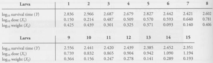
In an experiment to describe the toxic action of a certain chemical on silkworm larvae, the relationship of log10 dose and log10 larva weight to log10 survival time was sought. The data, obtained by feeding each larva a precisely measured dose of the chemical in an aqueous solution and then
An experiment to evaluate the effects of certain variables on soil erosion was performed on 10-foot-square plots of sloped farmland subjected to 2 inches of artificial rain applied over a 20-minute period. The data and related ANOVA table are as follows:a. Compute R2, and comment on the fit of the
In a study by Yoshida (1961), the oxygen consumption of wireworm larva groups was measured at five temperatures. The rate of oxygen consumption per larva group (in milliliters per hour)€”the dependent variable€”was transformed to 0.5 less than the common logarithm. Another
Use the data of Problem 1 in Chapter 8 to answer the following questions. a. Conduct the overall F tests for significant regression for the three models in Problem 1 of Chapter 8. Be sure to state the null and alternative hypotheses for each test and interpret each result. b. Based on your results
Data on sales revenue Y, television advertising expenditures X1, and print media advertising expenditures X2 for a large retailer for the period 1988-1993 were given in Problem 11 of Chapter 8. Use the computer output for that problem, along with the additional portions of the output shown here, to
Use the computer output for the radial keratotomy data of Problem 12 in Chapter 8, along with the additional output here, to answer the following questions.a. Perform the overall F test for the regression of Y on both independent variables. Interpret your result.b. Perform variables-added-in-order
Use the computer output for the Business Week magazine data of Problem 13 in Chapter 8, as well as the additional output here, to answer the following questions.a. Perform the overall F test for the regression of Y on both independent variables, X2 and X1. Interpret your result.b. Perform
This problem refers to the 1990 Census data presented in Problem 19 of Chapter 5 and in Problem 14 of Chapter 8.Use the computer output from Problem 14 of Chapter 8, along with the additional output shown here, to answer the following questions about the regression of OWN-EROCC on OWNCOST and
This problem refers to the pond ecology data of Chapter 5, Problem 20.a. Perform the overall F test for the multiple regression of copepod count on zooplankton and phytoplankton counts.b. Perform variables-added-in-order tests for both independent variables, with zoo-plankton count added first.c.
Consider once again the nutritional deficiency example and Model 4 from Chapter 8. In Section 9.6.5, the parameter L = (β1 + β2) associated with one-unit increases in height and age was considered, and a 95% confidence interval for this linear function was computed. For this problem, we now
The hypothetical study of two drugs A and B designed to lower systolic blood pressure has now been conducted, using a design where individuals are randomly assigned to take specific doses of both drugs. The researchers would like to know if 5 mg increases in each drug can decrease systolic blood
The numerical output in Section 9.7 was useful for answering questions (a)-(c) in the BRFSS example, but not every significance test about the independent variables can be performed using this single model's results. Which tests of hypotheses about the three predictors cannot be conducted using the
Use the information given in Problem 2 of Chapter 8, as well as the computer output given here, to answer the following questions about the data from that problem.a. Conduct overall regression F tests for these three models: Y regressed on X1 and X2; Y regressed on X1 alone; and Y regressed on X2
A psychologist examined the regression relationship between anxiety level (Y)€” measured on a scale ranging from 1 to 50, as the average of an index determined at three points in a 2-week period€”and the following three independent variables: X1 = systolic blood pressure; X2 = IQ; and X3 =
An educator examined the relationship between the number of hours devoted to reading each week (Y) and the independent variables social class (X1), number of years of school completed (X2), and reading speed (X3), in pages read per hour. The following ANOVA table was obtained from a stepwise
An experiment was conducted regarding a quantitative analysis of factors found in high-density lipoprotein (HDL) in a sample of human blood serum. Three variables thought to be predictive of, or associated with, HDL measurement (Y) were the total cholesterol (X1) and total triglyceride (X2)
Use the results from Problem 3 in Chapter 8, as well as the computer output given here, to answer the following questions about the data from that problem.a. Conduct overall regression F tests for these three models: Y regressed on weight and age; Y regressed on weight alone; and Y regressed on age
Use the results from Problem 4 in Chapter 8, as well as the computer output given here, to answer the following questions about the data from that problem.a. Conduct the overall regression F test for the model where Y is regressed on X1, X2, and X3. Use α = .05. Interpret your
The following ANOVA table is based on the data discussed in Problem 5 of Chapter 8. Use α = .05.a. Provide a test to compare the following two models: Y = β0 + β1X1 + β2X2 + β3X3 + E and Y = β0 + β1X1 + E b.
Residential real estate prices are thought to depend, in part, on property size and number of bedrooms. The house size X1 (in hundreds of square feet), number of bedrooms X2, and house price Y (in thousands of dollars) of a random sample of houses in a certain county were observed. The resulting
The correlation matrix obtained for the variables SBP (Y), AGE (X1), SMK (X2), and QUET (X3), using the data from Problem 2 in Chapter 5, is given bya. Based on this matrix, which of the independent variables AGE, SMK, and QUET explains the largest proportion of the total variation in the dependent
For the data discussed in Problem 6, provide numerical values for the following quantities: a. r2YX1 b. R2Y|X1, X2 c. R2Y|X1, X2, X3 d. r2YX3 | X1, X2 e. r2YX2 | X1
Use the results in Problem 7 to answer the following questions. a. Provide a numerical value for r2YX1|X2, X3. b. Which two models should you compare in testing whether the correlation in part (a) is zero in the population? c. Provide a numerical value for r2YX1. d. What does the difference between
The accompanying SAS computer output relates to the house price data of Problem 10 in Chapter 8. Use this output and, if necessary, the output associated with Problem 9 in Chapter 9 to answer the following questions.a. Determine r2Y|X1,X2, the squared multiple correlation between house price (Y)
The accompanying SAS computer output relates to the sales revenue data from Problem 11 in Chapter 8. Use this output and, if necessary, the output for Problem 10 in Chapter 9 to answer the following questions.a. Determine r2Y|X1,X2, the squared multiple correlation between sales revenue (Y) and the
The accompanying SAS computer output relates to the radial keratotomy data from Problem 12 in Chapter 8. Use this output and, if necessary, the output from Problem 11 in Chapter 9 to answer the following questions.a. Determine r2Y|X1,X2, the squared multiple correlation between change in refractive
The accompanying SAS computer output relates to the Business Week data from Problem 13 in Chapter 8. Use this output and, if necessary, the output from Problem 12 in Chapter 9 to answer the following questions.a. Determine r2Y|X2,X3, the squared multiple correlation between the yield (Y) and the
The accompanying SAS computer output relates to the 1990 Census data from Problem 14 in Chapter 8. Use this output and, if necessary, the output from Problem 13 in Chapter 9 to answer the following questions.a. Determine r2Y|X1,X2, the squared multiple correlation between the rate of owner
This problem refers to the pond ecology data of Chapter 5, Problem 20. a. Determine the squared multiple correlation for the regression of copepod count on zooplankton and phytoplankton counts. b. Determine the partial correlation between each independent variable in (a) and copepod count,
An (equivalent) alternative to performing a partial F test for the significance of adding a new variable to a model while controlling for variables already in the model is to perform a t test using the appropriate partial correlation coefficient. If the dependent variable is Y, the independent
a. Using the information provided in Problem 2 of Chapter 9, determine the proportion of residual variation that is explained by the addition of X2 to a model already containing X1; that is, computeb. How is the formula given in part (a) related to the partial correlation rYX2|X1?c. Test the
Refer to Problem 7 of Chapter 9 to answer the following questions about the relationship of homicide rate (Y) to city population size (X1), percentage of families with yearly incomes less than $5,000 (X2), and unemployment rate (X3).a. Determine the squared partial correlations r2YX1|X3 and
Using the ANOVA table given in Problem 8 of Chapter 9, which deals with the regression relationship of 12th-grade mean verbal SAT scores (Y) to per pupil expenditures (X1), percentage of teachers with advanced degrees (X2), and pupil-teacher ratio (X3), test the following null hypotheses:a. H0:
Using the following ANOVA table based on data in Problem 6 of Chapter 8 about the regression relationship of respiratory cancer mortality rates (Y) to air pollution index (X1), mean age (X2), and percentage of workforce employed in a certain industry (X3), test the following hypotheses:a. H0:
Refer to the following ANOVA tables and to SAS output given here (from data in Problem 8 of Chapter 8) to answer the following questions dealing with factors related to soil erosion.a. Using the accompanying SAS output, compute rYX2|X1 and rYX3|X1.b. Based on your results in part (a), which
Use the computer results from Problem 9 of Chapter 8 to answer the following questions. a. Test H0: pYX1 = 0 and H0: pYX2 = 0. b. Test H0: pYX1|X2 = 0 and H0: pYX2|X1 = 0. c. Based on your results in parts (a) and (b), which variables (if any) should be included in the regression model, and what is
Use the correlation matrix from Problem 1 to answer the following questions. a. Compute the semipartial rSBP(SMK|AGE). b. Compute the semipartial rSMK(SBP|AGE). c. Compare these correlations to the (full) partial rSBP, SMK|AGE computed in Problem 1.
Consider the numerical examples given in Section 8.8 of Chapter 8, involving assessment of the relationship of the independent variables HGT, AGE, and (AGE)2 to the dependent variable WGT. Suppose that HGT is the independent variable of primary concern, so interest lies in evaluating the
Refer to the Business Week magazine data in Problem 13 of Chapter 8. The relationships among the yield (Y), 1989 rank (X2), and P-E ratio (X3) were studied in that problem using a random sample of data from the magazine's compilation of information on the top 1,000 companies. The results of the
Let us return once more to the body-mass index (BMI) example for the BRFSS data. We now extend the models involving the explanatory factors of drinking frequency, age, and sleep quality in Chapters 8-9 to consider a model that includes all first-order product terms involving these three factors.
Consider the following computer results, which describe regression analyses involving two independent variables X1 and X2 and a dependent variable Y. Assume that your goal is to assess the relationship of X1 with Y, controlling for the possible confounding effects of X2.a. Using an appropriate
a-c. Consider the accompanying computer results, which describe regression analyses involving two independent variables X1 and X2 and a dependent variable Y (using a different data set from the one used in Problem 2). Answer the same questions as in Problem 2 for this new printout.d. What does this
A regression analysis of data on n = 53 males considered the following variables:Y = SBPSL (estimated slope based on the straight-line regression of an individual's blood pressure over time)X1 = SBP1 (initial blood pressure)X2 = RW (relative weight)X3 = X1X2 = SR (product of SBP1 and RW)The
An experiment involved a quantitative analysis of factors found in high-density lipoprotein (HDL) in a sample of human blood serum. Three variables thought to be predictive of or associated with HDL measurement (Y) were the total cholesterol (X1) and total triglyceride (X2) concentrations in the
Use the computer output from Problem 10 in Chapter 8 and from Problem 16 in Chapter 5 to answer the following questions. (Assume that no interaction occurs between house size [X1] and number of rooms [X2].) a. Does the number of rooms (X2) confound the relationship between house price (Y) and house
Use the output from Problem 11 in Chapter 8 and the output given here to answer the following questions. (Assume that no interaction occurs between TV advertising expenditure [X1] and print advertising expenditure [X2].)a. Does the print advertising expenditure confound the relationship between
Use the computer output from Problem 12 in Chapter 8 and the output given hereto answer the following questions.a. State the model that relates change in refraction (Y) to baseline refraction (X1), baseline curvature (X2), and the interaction of X1 and X2. Is the partial F test for the interaction
Refer to the data in Problem 19 of Chapter 5. The relationship between the rate of owner occupancy of housing units (OWNEROCC) and the median monthly ownership costs (OWNCOST) was studied in that problem in connection with a random sample of data from 26 Metropolitan Statistical Areas (MSAs). The
Using the data from Problem 2 in Chapter 5 and/or the SAS output given here, answer the following questions about the separate straight-line regressions of SBP on QUET for smokers (SMK = 1) and nonsmokers (SMK = 0).a. Determine the least-squares line of SBP (Y) on QUET (X) separately for smokers
The results presented in the following tables are based on data from a study by Gruber (1970) to determine how and to what extent changes in blood pressure over time depend on initial blood pressure (at the beginning of the study), the sex of the individual, and the relative weight of the
For the data from Problem 2 in this chapter, address the following questions, using the information provided in the accompanying SAS output.a. State the regression model that incorporates the straight-line models for each group of countries.b. Determine and plot the separate fitted straight lines,
Using the information given here, answer the same questions as in Problem 11 about the regression of height (Y) on age (X) for children in one of two diet categories. (This problem is based on the data in Problem 3.)In Problem 11a. State the regression model that incorporates the straight-line
In Gruber's (1970) study of n = 104 individuals (discussed in Problem 10), the relationship between blood pressure change (SBPSL) and relative weight (RW), controlling for initial blood pressure (SBP1), was compared for three different geographical backgrounds and for three different psychosocial
The Environmental Protection Agency conducted an experiment to assess the characteristics of sampling procedures designed to measure the suspended particulate concentration (X) in a particular city. At each of two distinct locations (designated as location 1 and location 2), two identical sampling
A biologist compared the effect of temperature for each of two media on the growth of human amniotic cells in a tissue culture. The data shown in the following table were obtained.a. Assuming that a parabolic model is appropriate for describing the relationship between Y and X for each medium,
Answer the following questions using the accompanying SPSS output, which is based on data on the growth rates (Y) of depleted chicks at different (log) dosage levels (X) of vitamin B for males and females.a. Define a single multiple regression model that incorporates different straight-line models
Market research was conducted for a national retail company to compare the relationship between sales and advertising during the warm spring and summer seasons as compared with the cool fall and winter seasons. The data shown in the following table were collected over a period of several years.a.
A testing laboratory studies and compares the relationship between tire tread wear per 1,000 miles (Y) and average driving speed (X) for two competing tire types (denoted A and B). The data shown in the following table were collected for a random sample of 20 tires, 10 of A and 10 of B.a. Identify
A random sample of data was collected on residential sales in a large city. The following table shows the sales price Y (in $ 1,000s), area X1 (in hundreds of square feet), number of bedrooms X2, total number of rooms X3, age X4 (in years), and location (dummy variables Z1 and Z2, defined as
A topic of major concern to demographers and economists is the effect of a high fertility rate on per capita income. The first two accompanying tables display values of per capita income (PCI) and population percentage under age 15 (YNG) for a hypothetical sample of developing countries in Latin
In Problem 19 in Chapter 5 and Problem 14 in Chapter 8, data from the 1990 Census for 26 randomly selected Metropolitan Statistical Areas (MSAs) were discussed. Of interest were factors potentially associated with the rate of owner occupancy of housing units. The following three variables were
This problem involves the PERK study data discussed in Problem 12 in Chapter 8. Suppose that we want to compare the relationship between changes in refraction five years after surgery and baseline refractive error, for males and females. To this end, we define the following dummy variable:a. State
A team of anthropologists and nutrition experts investigated the influence of protein content in diet on the relationship between AGE and height (HT) for New Guinean children. The first two accompanying tables display values of HT (in centimeters) and AGE for a hypothetical sample of children with
For the data involving regression of DI (Y) on IQ (X) in Problem 4 in Chapter 5, assume that the sample of 17 observations (with the outlier removed) consists of males only. Now suppose that another sample of observations on DI (Y) and IQ (X) has been obtained for 14 females. The information needed
Assume that the data involving the regression of VOTE (Y) on TVEXP (X) in Problem 5 in Chapter 5 came from congressional districts in New York. Now, suppose that researchers selected a second sample of 17 congressional districts in California and recorded the same information. The following table
The data in the following table represent four-week growth rates for depleted chicks at different dosage levels of vitamin B, by sex.Use the information provided in the next table to answer the following questions.a. Determine the dose-response straight lines separately for each sex, and plot them
The results in the first of the following tables were obtained in a study of the amount of energy metabolized by two similar species of birds under constant temperature. Information based on separate straight-line fits to each data set is summarized in the second table.a. Plot the least-squares
In Problem 1, separate straight-line regressions of SBP on QUET were compared for smokers (SMK = 1) and nonsmokers (SMK = 0).a. Define a single multiple regression model that uses the data for both smokers and nonsmokers and that defines straight-line models for each group with possibly differing
Use the computer output shown next to compare the separate regressions of SBP on AGE and QUET for smokers and nonsmokers (based on the data from Problem 2 in Chapter 5), as follows.a. State the appropriate regression model, simultaneously incorporating equations for both smokers and nonsmokers.b.
Problem 8 in Chapter 12 involved comparing straight-line regression fits of SBP on QUET for smokers and nonsmokers, and it was found that these straight lines could be considered parallel. Use results based on that problem and the computer output given next (and the fact that the overall sample
Repeat Problem 9 using LN_BLDTL as the dependent variable.Problem 9This problem involves data from Problem 15 in Chapter 5. Treat LN_BRNTL as the dependent variable and dosage level of toluene (PPM_TOLU) as a categorical predictor (four levels). The experimenter wanted to explore the possibility of
a. How would you compute appropriate cross-product terms for testing the interaction of WEIGHT and dosage level of toluene for Problem 9? b. State the appropriate regression model. c. State the null hypothesis (of no interaction) in terms of regression coefficients.
Refer to the residential sales data in Problem 19 in Chapter 12. Use the computer output given below to answer the following questions.a. State an ANACOVA regression model that can be used to compare outer suburbs with other locations (intown and inner suburbs), controlling for age.b. Identify the
A company wants to compare three different point-of-sale promotions for its snack foods. The three promotions arePromotion 1: Buy two items, get a third free.Promotion 2: Mail in a rebate for $1.00 with any $2.00 purchase.Promotion 3: Buy reduced-price multipacks of each snack food.The company is
In Problem 19 in Chapter 5 and Problem 14 in Chapter 8, data from the 1990 Census for 26 randomly selected Metropolitan Statistical Areas (MSAs) were discussed. Of interest were factors potentially associated with the rate of owner occupancy of housing units. The following three variables were
This problem refers to the radial keratotomy study data from Problem 12 in Chapter 8. Suppose that we want to compare the average change in refraction for males and females, controlling for baseline refractive error and baseline curvature. To this end, we define the following dummy variable:a.
For the BRFSS example discussed in Section 13.6, there are a number of inference-making procedures that may be conducted about the joint effects of the two exposure variables exercise and tobacco_now. Using the output in Section 13.6 and below for the analyses of 1,048 individuals, do the
In Section 13.6, adjusted mean BMI values were obtained for the two nominal variables exercise and tobacco_now. A drawback of the approach used is that these four adjusted means were estimated for the four combinations of these two factors considered simultaneously, leaving one without adjusted
a.-d. Answer the same questions as in parts (a) through (d) in Problem 1 regarding an analysis of covariance designed to control for both AGE and QUET. (AGE = 53.250.) Use the results from Problem 9 in Chapter 12.e. Is it necessary to control for both AGE and QUET as opposed to controlling just one
In an experiment conducted at the National Institute of Environmental Health Sciences, the absorption (or uptake) of a chemical by a rat on one of two different diets, I or II, was known to be affected by the weight (or size) of the rat. A completely randomized design utilizing four rats on each
A political scientist developed a questionnaire to determine political tolerance scores (Y) for a random sample of faculty members at her university. She wanted to compare mean scores adjusted for age (X) in each of three categories: full professors, associate professors, and assistant professors.
A psychological experiment was performed to determine whether in problem-solving dyads containing one male and one female, "influencing" behavior depended on the sex of the experimenter. The problem for each dyad was a strategy game called "Rope a Steer," which required 20 separate decisions about
An experiment was conducted to compare the effects of four different drugs (A, B, C, and D) in delaying atrophy of denervated muscles. A certain leg muscle in each of 48 rats was deprived of its nerve supply by surgical severing of the appropriate nerves. The rats were then put randomly into four
Trough urine samples were analyzed for sodium content for each of two collection periods, one before and one after administration of Mercuhydrin, for each of 30 dogs. The experimenter used 7 dogs as a control group for the study; these dogs were not administered the drug, but their urine samples
Consider again the data in Problem 4.a. How would you compute appropriate cross-product variables to allow testing of whether an interaction exists between age and faculty rank?b. State the associated regression model.c. Using a computer, fit the model. Provide estimates of the regression
This problem involves data from Problem 15 in Chapter 5. Treat LN_BRNTL as the dependent variable and dosage level of toluene (PPM_TOLU) as a categorical predictor (four levels). The experimenter wanted to explore the possibility of using WEIGHT as a control variable.a. State the appropriate
a.-c. Consider the data of Problem 15, Chapter 5. For the model with BLOODTOL as the response and PPM_TOLU as the predictor, repeat (a) through (c) of Problem 1.
a.-c. Repeat Problem 15 using LN_BLDTL as the response and LN_PPMTL as the predictor.d. Which approach—using the original variables or using the logged variables—leads to fewer diagnostic problems?
a.-c. Repeat Problem 15 using BLOODTOL as the response and BRAINTOL as the predictor.
a.-d. Repeat Problem 16 using LN_BLDTL as the response and LN_BRNTL as the predictor.
The data in the following table come from an article by Bethel et al. (1985). All subjects are asthmatics. For the model with FEV1 as the response and HEIGHT, WEIGHT, and AGE as the predictors,a. Examine a plot of the studentized or jackknife residuals versus the predicted values. Are any
a.-c. Repeat Problem 1 using log10(dry weight) as the response. Problem 1 Consider the data of Problem 1, Chapter 5. For the model with dry weight as the response and age as the predictor, a. Examine a plot of the studentized or jackknife residuals versus the predicted values. Are any regression
This time including SEX as a predictor (coded SEX = 1 if female, SEX = 0 if male).a. Examine a plot of the studentized or jackknife residuals versus the predicted values. Are any regression assumption violations apparent? If so, suggest possible remedies.b. Examine numerical descriptive statistics,
Repeat Problem 20, this time including three interactions: SEX and AGE, SEX and HEIGHT, and SEX and WEIGHT.
Showing 50300 - 50400
of 88243
First
497
498
499
500
501
502
503
504
505
506
507
508
509
510
511
Last
Step by Step Answers
.png)
-1.png)
-2.png)
-1.png)
-2.png)
-1.png)
-2.png)
-3.png)
-1.png)
-2.png)
.png)
.png)
.png)
.png)
.png)
.png)
.png)
.png)
-1.png)
-2.png)
.png)
.png)
-1.png)
.png)
-1.png)
-2.png)
.png)
.png)
.png)
.png)
.png)
-1.png)
-2.png)
.png)
.png)
-1.png)
-2.png)
-3.png)
.png)
.png)
.png)
-1.png)
-2.png)
-1.png)
-2.png)
.png)
.png)
.png)
.png)
-1.png)
-2.png)
-1.png)
-2.png)
.png)
.png)
.png)
-2.png)
-3.png)
-1.png)
-2.png)
.png)
-1.png)
-2.png)
-1.png)
-2.png)
-1.png)
-2.png)
-1.png)
-2.png)
-3.png)
-1.png)
-2.png)
-2.png)
-3.png)
-1.png)
-2.png)
-3.png)
.png)
.png)
-1.png)
-2.png)
-2.png)
-3.png)
.png)
.png)
.png)
-1.png)
-2.png)
-1.png)
-2.png)
-3.png)
-2.png)
-2.png)
-3.png)
.png)
.png)
-1.png)
-2.png)
-1.png)
-2.png)
-1.png)
-2.png)
-3.png)
-1.png)
-2.png)
-3.png)
.png)
.png)

