New Semester Started Get 50% OFF Study Help! --h --m --s Claim Now

Question Answers

Textbooks

Find textbooks, questions and answers

Oops, something went wrong!

Change your search query and then try again

Result Not Found

Books FREE
Study Help
Tutors
AI Study Planner NEW
Sell Books

Search
Sign In
Register

study help
mathematics
statistics

Mathematical Interest Theory 3rd Edition Leslie Jane, James Daniel, Federer Vaaler - Solutions

Among 198 smokers who underwent a "sustained care" program, 51 were no longer smoking after six months. Among 199 smokers who underwent a "standard care" program, 30 were no longer smoking after six months (based on data from "Sustained Care Intervention and Post-discharge Smoking Cessation Among
Data Set 12 “Passive and Active Smoke” in Appendix B includes cotinine levels measured in a group of nonsmokers exposed to tobacco smoke (n = 40, x = 60.58 ng/mL, s = 138.08 ng/mL) and a group of nonsmokers not exposed to tobacco smoke (n = 40, x̅ = 16.35 ng/mL, s = 62.53 ng/ mL). Cotinine is
a. Use a 0.05 significance level to test the claim that two samples of course evaluation scores are from populations with the same mean. Use these summary statistics: Female professors:n = 40, x̅ = 3.79, s = 0.51; male professors: n = 53, x̅ = 4.01, s = 0.53. (Using the raw data in Data Set 17
A study of seat belt use involved children who were hospitalized after motor vehicle crashes. For a group of 123 children who were wearing seat belts, the number of days in intensive care units (ICU) has a mean of 0.83 and a standard deviation of 1.77. For a group of 290 children who were not
Weights of quarters are carefully considered in the design of the vending machines that we have all come to know and love. Data Set 29 "Coin Weights" in Appendix B includes weights of a sample of pre-1964 quarters (n = 40, x̅ = 6.19267 g, s = 0.08700 g) and weights of a sample of post-1964
Data Set 11 “Alcohol and Tobacco in Movies” in Appendix B includes lengths of times (seconds) of tobacco use shown in animated children’s movies. For the Disney movies, n = 33, x̅ = 61.6 sec, s = 118.8 sec. For the other movies, n = 17, x = 49.3 sec, s = 69.3 sec. The sorted times for the
Listed below are student evaluation scores of female professors and male professors from Data Set 17 "Course Evaluations" in Appendix B. Test the claim that female professors and male professors have the same mean evaluation ratings. Does there appear to be a difference?
When the author visited Dublin, Ireland (home of Guinness Brewery employee William Gosset, who first developed the t distribution), he recorded the ages of randomly selected passenger cars and randomly selected taxis. The ages can be found from the license plates. (There is no end to the fun of
Listed below are time intervals (min) between eruptions of the Old Faithful geyser. The "recent" times are within the past few years, and the "past" times are from 1995. Does it appear that the mean time interval has changed? Is the conclusion affected by whether the significance level is 0.05 or
Assume that the two samples are independent simple random samples selected from normally distributed populations, and do not assume that the population standard deviations are equalMany students have had the unpleasant experience of panicking on a test because the first question was exceptionally
Refer to Data Set 24 "Word Counts" and use the measured word counts from men in the third column and the measured word counts from women in the fourth column. Use a 0.05 significance level to test the claim that men talk less than women.Use the indicated Data Sets in Appendix B. The complete data
Repeat Exercise 10 “Heights of Fathers and Sons” using all of the heights of fathers and sons listed in Data Set 5“Family Heights” in Appendix B.
Refer to Data Set 4"Births" and use the birth weights of boys and girls. Test the claim that at birth, girls have a lower mean weight than boys.Use the indicated Data Sets in Appendix B. The complete data sets can be found at www.TriolaStats.com. Assume that the two samples are independent simple
Refer to Data Set 4"Births" and use the "lengths of stay" for boys and girls. A length of stay is the number of days the child remained in the hospital. Test the claim boys and girls have the same mean length of stay.Use the indicated Data Sets in Appendix B. The complete data sets can be found at
Repeat Exercise 12 “IQ and Lead” by assuming that the two population standard deviations are equal, so σ1 = σ2. Use the appropriate method from Part 2 of this section. Does pooling the standard deviations yield results showing greater significance?
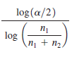
In Exercise 20 "Blanking Out on Tests," using the "smaller of n1 - 1 and n2 - 1" for the number of degrees of freedom results in df = 15. Find the number of degrees of freedom using Formula 9-1. In general, how are hypothesis tests and confidence intervals affected by using Formula 9-1 instead of
An experiment was conducted to test the effects of alcohol. Researchers measured the breath alcohol levels for a treatment group of people who drank ethanol and another group given a placebo. The results are given below (based on data from "Effects of Alcohol Intoxication on Risk Taking, Strategy,
For Example 1 on page 431, we used df = smaller of n1 - 1 and n2 - 1, we got df = 11, and the corresponding critical values are t = ( 2.201. If we calculate df using Formula 9-1, we get df = 19.063, and the corresponding critical values are (2.093. How is using the critical values of t = (2.201
Data Set 26 “Cola Weights and Volumes” in Appendix B includes weights (lb) of the contents of cans of Diet Coke (n = 36, x̅ = 0.78479 lb, s = 0.00439 lb) and of the contents of cans of regular Coke (n = 36, x = 0.81682 lb, s = 0.00751 lb).a. Use a 0.05 significance level to test the
Data Set 26 “Cola Weights and Volumes” in Appendix B includes volumes of the contents of cans of regular Coke (n = 36, x̅ = 12.19 oz, s = 0.11 oz) and volumes of the contents of cans of regular Pepsi (n = 36, x = 12.29 oz, s = 0.09 oz).a. Use a 0.05 significance level to test the claim that
Researchers from the University of British Columbia conducted trials to investigate the effects of color on creativity. Subjects with a red background were asked to think of creative uses for a brick; other subjects with a blue background were given the same task. Responses were scored by a panel
Researchers from the University of British Columbia conducted a study to investigate the effects of color on cognitive tasks. Words were displayed on a computer screen with background colors of red and blue. Results from scores on a test of word recall are given below. Higher scores correspond to
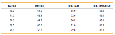
Listed below are heights (in.) of fathers and their first sons. The data are from a journal kept by Francis Galton. (See Data Set 5"Family Heights" in Appendix B.) Use a 0.05 significance level to test the claim that there is no difference in heights between fathers and their first sons.
Listed below are "attribute" ratings made by participants in a speed dating session. Each attribute rating is the sum of the ratings of five attributes (sincerity, intelligence, fun, ambition, shared interests). The listed ratings are from Data Set 18"Speed Dating" in Appendix B. Use a 0.05
Listed below are "attractiveness" ratings made by participants in a speed dating session. Each attribute rating is the sum of the ratings of five attributes (sincerity, intelligence, fun, ambition, shared interests). The listed ratings are from Data Set 18"Speed Dating." Use a 0.05 significance
A study was conducted to investigate the effectiveness of hypnotism in reducing pain. Results for randomly selected subjects are given in the accompanying table (based on "An Analysis of Factors That Contribute to the Efficacy of Hypnotic Analgesia," by Price and Barber, Journal of Abnormal
As part of the National Health and Nutrition Examination Survey, the Department of Health and Human Services obtained self-reported heights (in.) and measured heights (in.) for males aged 12-16. Listed below are sample results. Construct a 99% confidence interval estimate of the mean difference
Repeat Exercise 6 "Heights of Presidents" using all of the sample data from Data Set 15 "Presidents" in Appendix B.Use the indicated Data Sets in Appendix B. The complete data sets can be found at www.TriolaStats.com. Assume that the paired sample data are simple random samples and the differences
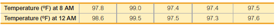
Repeat Exercise 7 "Body Temperatures" using all of the 8 AM and 12 AM body temperatures on Day 2 as listed in Data Set 3Use the indicated Data Sets in Appendix B. The complete data sets can be found at www.TriolaStats.com. Assume that the paired sample data are simple random samples and the
Listed below are body temperatures from five different subjects measured at 8 AM and again at 12 AM (from Data Set 3“Body Temperatures” in Appendix B). Find the values of d and d̅. In general, what does μd represent?
Listed below are the numbers of words spoken in a day by each member of six different couples. The data are randomly selected from the first two columns in Data Set 24Data Set 24"Word Counts" in Appendix B. a. Use a 0.05 significance level to test the claim that among couples, males speak fewer
Listed below are heights (in.) of mothers and their first daughters. The data are from a journal kept by Francis Galton. (See Data Set 5 "Family Heights" in Appendix B.) Use a 0.05 significance level to test the claim that there is no difference in heights between mothers and their first
Listed below are heights (in.) of fathers and their first sons. The data are from a journal kept by Francis Galton. (See Data Set 5 "Family Heights" in Appendix B.) Use a 0.05 significance level to test the claim that there is no difference in heights between fathers and their first sons.Repeat
Use the listed paired sample data, and assume that the samples are simple random samples and that the differences have a distribution that is approximately normal.Listed below are "attribute" ratings made by participants in a speed dating session. Each attribute rating is the sum of the ratings of
Listed below are "attractiveness" ratings made by participants in a speed dating session. Each attribute rating is the sum of the ratings of five attributes (sincerity, intelligence, fun, ambition, shared interests). The listed ratings are from Data Set 18 "Speed Dating." Use a 0.05 significance
Refer to Data Set 3"Body Temperatures" in Appendix B and use all of the matched pairs of body temperatures at 8 AM and 12 AM on Day 1. When using a 0.05 significance level for testing a claim of a difference between the temperatures at 8 AM and at 12 AM on Day 1, how are the hypothesis test results
a. If paired sample data (x, y) are such that the values of x do not appear to be from a population with a normal distribution, and the values of y do not appear to be from a population with a normal distribution, does it follow that the values of d̅ will not appear to be from a population with a
A popular theory is that presidential candidates have an advantage if they are taller than their main opponents. Listed are heights (cm) of presidents along with the heights of their main opponents (from Data Set 15"Presidents"). a. Use the sample data with a 0.05 significance level to test the
Use the listed paired sample data, and assume that the samples are simple random samples and that the differences have a distribution that is approximately normal.Listed below are body temperatures from seven different subjects measured at two different times in a day (from Data Set 3"Body
Listed below are the numbers of words spoken in a day by each member of six different couples. The data are randomly selected from the first two columns in Data Set 24"Word Counts" in Appendix B. a. Use a 0.05 significance level to test the claim that among couples, males speak fewer words in a day
Listed below are heights (in.) of mothers and their first daughters. The data are from a journal kept by Francis Galton. (See Data Set 5"Family Heights" in Appendix B.) Use a 0.05 significance level to test the claim that there is no difference in heights between mothers and their first daughters.
When the author visited Dublin, Ireland (home of Guinness Brewery employee William Gosset, who first developed the t distribution), he recorded the ages of randomly selected passenger cars and randomly selected taxis. The ages (in years) are listed below. Use a 0.05 significance level to test the
Listed below are student evaluation scores of female professors and male professors from Data Set 17 "Course Evaluations" in Appendix B. Use a 0.05 significance level to test the claim that female professors and male professors have evaluation scores with the same variation.
Listed below are time intervals (min) between eruptions of the Old Faithful geyser. The "recent" times are within the past few years, and the "past" times are from 1995. Does it appear that the variation of the times between eruptions has changed?
Many students have had the unpleasant experience of panicking on a test because the first question was exceptionally difficult. The arrangement of test items was studied for its effect on anxiety. The following scores are measures of "debilitating test anxiety," which most of us call panic or
Many students have had the unpleasant experience of panicking on a test because the first question was exceptionally difficult. The arrangement of test items was studied for its effect on anxiety. The following scores are measures of "debilitating test anxiety," which most of us call panic or
Many students have had the unpleasant experience of panicking on a test because the first question was exceptionally difficult. The arrangement of test items was studied for its effect on anxiety. The following scores are measures of "debilitating test anxiety," which most of us call panic or
If using the sample data in Data Set 1"Body Data" in Appendix B for a test of the claim that heights of men and heights of women have different variances, we find that s = 7.48296 cm for women and s = 7.10098 cm for men. a. Find the values of s21 and s22 and express them with appropriate units of
For the hypothesis test described in Exercise 2, the sample sizes are n1 = 147 and n2 = 153. When using the F test with these data, is it correct to reason that there is no need to check for normality because n1 > 30 and n2 > 30?
Researchers from the University of British Columbia conducted trials to investigate the effects of color on creativity. Subjects with a red background were asked to think of creative uses for a brick; other subjects with a blue background were given the same task. Responses were scored by a panel
Researchers from the University of British Columbia conducted trials to investigate the effects of color on the accuracy of recall. Subjects were given tasks consisting of words displayed on a computer screen with background colors of red and blue. The subjects studied 36 words for 2 minutes, and
Data Set 12“Passive and Active Smoke” includes cotinine levels measured in a group of smokers (n = 40, x̅ = 172.48 ng>mL, s = 119.50 ng>mL) and a group of nonsmokers not exposed to tobacco smoke (n = 40, x̅ = 16.35 ng>mL, s = 62.53 ng>mL). Cotinine is a metabolite of nicotine, meaning that
In the article "The Denomination Effect" by Priya Raghubir and Joydeep Srivastava, Journal of Consumer Research, Vol. 36, researchers reported results from studies conducted to determine whether people have different spending characteristics when they have larger bills, such as a $20 bill, instead
Construct the confidence interval that could be used to test the claim in Exercise 1. What feature of the confidence interval leads to the same conclusion from Exercise 1?
Listed below are heights (cm) randomly selected from the sample of women and heights (cm) randomly selected from the sample of men (from Data Set 1 "Body Data" in Appendix B). Use a 95% confidence level to estimate the magnitude of the difference between the mean height of women and the mean height
Use a 0.01 significance level with the sample data from Exercise 3 to test the claim that women have heights with a mean that is less than the mean height of men.
Listed below are the costs (in dollars) of flights from New York (JFK) to Los Angeles (LAX). Use a 0.01 significance level to test the claim that flights scheduled one day in advance cost more than flights scheduled 30 days in advance. What strategy appears to be effective in saving money when
Use the sample data given in Exercise 3 "Heights" and test the claim that women and men have heights with the same variation. Use a 0.05 significance level.
Use the following heights (in.) The data are matched so that each column consists of heights from the same family.a. Are the three samples independent or dependent? Why? b. Find the mean, median, range, standard deviation, and variance of the heights of the sons. c. What is the level of measurement
Braking Reaction Times: Confidence Intervals a. Construct a 99% confidence interval estimate of the mean braking reaction time of males, construct a 99% confidence interval estimate of the mean braking reaction time of females, then compare the results. b. Construct a 99% confidence interval
Construct a scatter plot of the father / son heights, then interpret it?
Use a 0.05 significance level to test the claim that differences between heights of fathers and their sons have a mean of 0 in?
Interpret the normal quantile plot of heights of fathers.
Listed below are sorted braking reaction times (in 1>10,000 sec) for male and female subjects (based on data from the RT-2S Brake Reaction Time Tester). Construct a histogram for the reaction times of males. Use a class width of 8 and use 28 as the lower limit of the first class. For the horizontal
The accompanying normal quantile plot is obtained by using the braking reaction times of females listed in Exercise 6. Interpret this graph.
Listed below are sorted braking reaction times (in 1>10,000 sec) for male and female subjects (based on data from the RT-2S Brake Reaction Time Tester). Construct a histogram for the reaction times of males. Use a class width of 8 and use 28 as the lower limit of the first class. For the horizontal
Listed below are sorted braking reaction times (in 1>10,000 sec) for male and female subjects (based on data from the RT-2S Brake Reaction Time Tester). Construct a histogram for the reaction times of males. Use a class width of 8 and use 28 as the lower limit of the first class. For the horizontal
Twenty different statistics students are randomly selected. For each of them, their body temperature (°C) is measured and their head circumference (cm) is measured. a. For this sample of paired data, what does r represent, and what does r represent? b. Without doing any research or calculations,
Listed below are numbers of Internet users per 100 people and numbers of Nobel Laureates per 10 million people (from Data Set 16 "Nobel Laureates and Chocolate" in Appendix B) for different countries. Is there sufficient evidence to conclude that there is a linear correlation between Internet users
Listed below are duration times (seconds) and time intervals (min) to the next eruption for randomly selected eruptions of the Old Faithful geyser in Yellowstone National Park. Is there sufficient evidence to conclude that there is a linear correlation between duration times and interval after
The "pizza connection" is the principle that the price of a slice of pizza in New York City is always about the same as the subway fare. Use the data listed below to determine whether there is a significant linear correlation between the cost of a slice of pizza and the subway fare.
Use CPI / subway data from the preceding exercise to determine whether there is a significant linear correlation between the CPI (Consumer Price Index) and the subway fare?
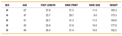
Police sometimes measure shoe prints at crime scenes so that they can learn something about criminals. Listed below are shoe print lengths, foot lengths, and heights of males (from Data Set 2 "Foot and Height" in Appendix B). Is there sufficient evidence to conclude that there is a linear
Use the paired foot length and height data from the preceding exercise. Is there sufficient evidence to conclude that there is a linear correlation between foot lengths and heights of males? Based on these results, does it appear that police can use foot length to estimate the height of a male?
Listed below are combined city-highway fuel economy ratings (in mi>gal) for different cars. The old ratings are based on tests used before 2008 and the new ratings are based on tests that went into effect in 2008. Is there sufficient evidence to conclude that there is a linear correlation between
Listed below are ages of Oscar winners matched by the years in which the awards were won (from Data Set 14 "Oscar Winner Age" in Appendix B). Is there sufficient evidence to conclude that there is a linear correlation between the ages of Best Actresses and Best Actors? Should we expect that there
Listed below are numbers of registered pleasure boats in Florida (tens of thousands) and the numbers of manatee fatalities from encounters with boats in Florida for each of several recent years. The values are from Data Set 10 "Manatee Deaths" in Appendix B. Is there sufficient evidence to conclude
Listed below are amounts of bills for dinner and the amounts of the tips that were left. The data were collected by students of the author. Is there sufficient evidence to conclude that there is a linear correlation between the bill amounts and the tip amounts? If everyone were to tip with the same
Media periodically discuss the issue of heights of winning presidential candidates and heights of their main opponents. Listed below are those heights (cm) from several recent presidential elections (from Data Set 15 "Presidents" in Appendix B). Is there sufficient evidence to conclude that there
Use all of the paired Internet/Nobel data listed in Data Set 16 "Nobel Laureates and Chocolate" in Appendix B? "Presidents" in Appendix B). Is there sufficient evidence to conclude that there is a linear correlation between heights of winning presidential candidates and heights of their main
If we find that there is a linear correlation between the concentration of carbon dioxide (CO2) in our atmosphere and the global mean temperature, does that indicate that changes in CO2 cause changes in the global mean temperature? Why or why not?
Use all of the paired duration/interval after times listed in Data Set 23.Use the data from Appendix B to construct a scatterplot, find the value of the linear correlation coefficient r, and find either the P-value or the critical values of r from Table A-6 using a significance level of Î± =
Use all of the shoe print lengths and heights of the 19 males from Data Set 2 "Foot and Height" in Appendix B?Use the data from Appendix B to construct a scatterplot, find the value of the linear correlation coefficient r, and find either the P-value or the critical values of r from Table A-6 using
Use all of the foot lengths and heights of the 19 males from Data Set 2 "Foot and Height" in Appendix B?Use the data from Appendix B to construct a scatterplot, find the value of the linear correlation coefficient r, and find either the P-value or the critical values of r from Table A-6 using a
Refer to Data Set 24 "Word Counts" in Appendix B and use the word counts measured from men and women in couple relationships listed in the first two columns of Data Set 24?
Refer to Data Set 21"Earthquakes" in Appendix B and use the depths and magnitudes from the earthquakes. Does it appear that depths of earthquakes are associated with their magnitudes?MAGNITUDE ________ DEPTH2.45 ................... 0.73.62 ................... 6.03.06 ................... 7.03.30
Fifty-four wild bears were anesthetized, and then their weights and chest sizes were measured and listed in Data Set 9 "Bear Measurements" in Appendix B; results are shown in the accompanying Stat-disk display. Is there sufficient evidence to support the claim that there is a linear correlation
The New York Times published the sizes (square feet) and revenues (dollars) of seven different casinos in Atlantic City. Is there sufficient evidence to support the claim that there is a linear correlation between size and revenue? Do the results suggest that a casino can increase its revenue by
Data Set 31 "Garbage Weight" in Appendix B includes weights of garbage discarded in one week from 62 different households. The paired weights of paper and glass were used to obtain the XLSTAT results shown here. Is there sufficient evidence to support the claim that there is a linear correlation
Find the best predicted Nobel Laureate rate for Japan, which has 79.1 Internet users per 100 people. How does it compare to Japan's Nobel Laureate rate of 1.5 per 10 million people?
Using the listed duration and interval after times, find the best predicted "interval after" time for an eruption with a duration of 253 seconds. How does it compare to an actual eruption with a duration of 253 seconds and an interval after time of 83 minutes?In each case, find the regression
Use the pizza costs and subway fares to find the best predicted subway fare, given that the cost of a slice of pizza is $3.00. Is the best predicted subway fare likely to be implemented?In each case, find the regression equation, letting the first variable be the predictor (x) variable. Find the
Use the CPI / subway fare data from the preceding exercise and find the best predicted subway fare for a time when the CPI reaches 500. What is wrong with this prediction?In each case, find the regression equation, letting the first variable be the predictor (x) variable. Find the indicated
Use the shoe print lengths and heights to find the best predicted height of a male who has a shoe print length of 31.3 cm. Would the result be helpful to police crime scene investigators in trying to describe the male?In each case, find the regression equation, letting the first variable be the
Use the foot lengths and heights to find the best predicted height of a male who has a foot length of 28 cm. Would the result be helpful to police crime scene investigators in trying to describe the male?In each case, find the regression equation, letting the first variable be the predictor (x)
Using the listed lemon / crash data, find the best predicted crash fatality rate for a year in which there are 500 metric tons of lemon imports. Is the prediction worthwhile?In each case, find the regression equation, letting the first variable be the predictor (x) variable. Find the indicated
Using the listed old / new mpg ratings, find the best predicted new mpg rating for a car with an old rating of 30 mpg. Is there anything to suggest that the prediction is likely to be quite good?In each case, find the regression equation, letting the first variable be the predictor (x) variable.
Using the listed actress / actor ages, find the best predicted age of the Best Actor given that the age of the Best Actress is 54 years. Is the result reasonably close to the Best Actor's (Eddie Redmayne) actual age of 33 years, which happened in 2015, when the Best Actress was Julianne Moore, who
Use the listed boat/manatee data. In a year not included in the data below, there were 970,000 registered pleasure boats in Florida. Find the best predicted number of manatee fatalities resulting from encounters with boats. Is the result reasonably close to 79, which was the actual number of
Using the bill / tip data, find the best predicted tip amount for a dinner bill of $100. What tipping rule does the regression equation suggest?In each case, find the regression equation, letting the first variable be the predictor (x) variable. Find the indicated predicted value by following the

Showing 75700 - 75800 of 88243

First
751
752
753
754
755
756
757
758
759
760
761
762
763
764
765
Last

Step by Step Answers

Services

Sitemap
Fun
Definitions
Become Tutor
Used Textbooks
Study Help Categories
Recent Questions
Expert Questions
Campus Wear
Sell Your Books

Company Info

Security
Copyrights
Privacy Policy
Terms & Conditions
SolutionInn Fee
Scholarship
Online Quiz
Give Feedback, Get Rewards

Get In Touch

About Us
Contact Us
Career
Jobs
FAQ
Student Discount
Campus Ambassador

Secure Payment

Download Our App

© 2026 SolutionInn. All Rights Reserved