New Semester
Started
Get
50% OFF
Study Help!
--h --m --s
Claim Now
Question Answers
Textbooks
Find textbooks, questions and answers
Oops, something went wrong!
Change your search query and then try again
S
Books
FREE
Study Help
Expert Questions
Accounting
General Management
Mathematics
Finance
Organizational Behaviour
Law
Physics
Operating System
Management Leadership
Sociology
Programming
Marketing
Database
Computer Network
Economics
Textbooks Solutions
Accounting
Managerial Accounting
Management Leadership
Cost Accounting
Statistics
Business Law
Corporate Finance
Finance
Economics
Auditing
Tutors
Online Tutors
Find a Tutor
Hire a Tutor
Become a Tutor
AI Tutor
AI Study Planner
NEW
Sell Books
Search
Search
Sign In
Register
study help
business
econometrics
Econometrics 1st Edition Bruce Hansen - Solutions
A two-step estimator such as (12.49) is b¯ Æ¡PniÆ1 cWicW0 i¢¡1 ¡PniÆ1 cWiYi¢where cWi Æ bA 0Zi and bA Æ¡Z0Z¢¡1 Z0X . Describe how to construct the jackknife estimator of variance of b¯.
Show that if the jackknife estimator of variance of b¯ is bV jack b¯, then the jackknife estimator of variance of bµ Æ a ÅC b¯ is bV jack bµÆC bV jack b¯C0.
Find the jackknife estimator of variance of the estimator b¹r Æ n¡1PniÆ1 Y r i for ¹r Æ E£Y r i¤.
Using the cps09mar dataset and the subsample of non-Hispanic Black individuals (race code = 2) and white individuals (race code = 1) test the hypothesis that the returns to education is common across groups.(a) Allow the return to education to vary across the four groups (white male, white female,
Using the cps09mar dataset and the subsample of non-Hispanic Black individuals (race code = 2) test the hypothesis that marriage status does not affectmean wages.(a) Take the regression reported in Table 4.1. Which variables will need to be omitted to estimate a regression for this subsample?(b)
In Section 8.12 we reported estimates from Mankiw, Romer and Weil (1992). We reported estimation both by unrestricted least squares and by constrained estimation, imposing the constraint that three coefficients (2nd , 3rd and 4th coefficients) sum to zero as implied by the Solow growth theory.Using
In a paper in 1963, Marc Nerlove analyzed a cost function for 145 American electric companies.Nerlov was interested in estimating a cost function: C Æ f (Q,PL,PF,PK) where the variables are listed in the table below. His data set Nerlove1963 is on the textbook website.(a) First, estimate an
The data set Invest1993 on the textbook website contains data on 1962 U.S. firms extracted from Compustat, assembled by Bronwyn Hall, and used in Hall and Hall (1993).The variables we use in this exercise are in the table below. The flow variables are annual sums. The stock variables are beginning
Do a Monte Carlo simulation. Take the model Y Æ ®Å X¯Åe with E[Xe] Æ 0 where the parameter of interest is µ Æ exp(¯). Your data generating process (DGP) for the simulation is: X isU[0,1], e » N(0,1) is independent of X, and n Æ 50. Set ® Æ 0 and ¯ Æ 1. Generate B Æ 1000 independent
Let T be a test statistic such that under H0, T ¡!dÂ23. Since P£Â23È 7.815¤Æ 0.05, an asymptotic 5% test of H0 rejects when T È 7.815. An econometrician is interested in the Type I error of this test when n Æ 100 and the data structure is well specified. She performs the followingMonte
You have a random sample from the model Y Æ X¯1 Å X2¯2 Åe with E[e j X] Æ 0 where Y is wages (dollars per hour) and X is age. Describe how you would test the hypothesis that the expected wage for a 40-year-old worker is $20 an hour.
Take themodel Y Æ X1¯1 ÅX2¯2 ÅX3¯3 ÅX4¯4 Åe with E[Xe] Æ 0. Describe how to test against 1 B3 Ho: 2 B4 B1, B3 H: B2 PA
You are reading a paper, and it reports the results from two nested OLS regressions:You are curious if the estimate b¯2 is statistically different from the zero vector. Is there away to determine an answer fromthis information? Do you have to make any assumptions (beyond the standard regularity
An economist estimates Y Æ X0 1¯1 Å X2¯2 Åe by least squares and tests the hypothesis H0 : ¯2 Æ 0 against H1 : ¯2 6Æ 0. Assume ¯1 2 Rk and ¯2 2 R. She obtains a Wald statistic W Æ 0.34. The sample size is n Æ 500.(a) What is the correct degrees of freedom for the Â2 distribution to
The observed data is {Yi ,Xi ,Zi } 2 R£Rk£R`, k È 1 and ` È 1, i Æ 1, ...,n. An econometrician first estimates Yi Æ X0 ib¯Å bei by least squares. The econometrician next regresses the residual bei on Zi , which can be written as bei Æ Z0 i e°Å eui .(a) Define the population parameter °
You have two regressors X1 and X2 and estimate a regression with all quadratic terms included Y Æ ®Å¯1X1 ů2X2 ů3X2 1 ů4X2 2 ů5X1X2 Åe.One of your advisors asks: Can we exclude the variable X2 from this regression?How do you translate this question into a statistical test? When
Consider two alternative regression modelswhere X1 and X2 have at least some different regressors. (For example, (9.21) is a wage regression on geographic variables and (2) is a wage regression on personal appearance measurements.) You want to know if model (9.21) or model (9.22) fits the data
You are at a seminar where a colleague presents a simulation study of a test of a hypothesis H0 with nominal size 5%. Based on B Æ 100 simulation replications under H0 the estimated size is 7%.Your colleague says: “Unfortunately the test over-rejects.”(a) Do you agree or disagree with your
Take the model Y Æ X0¯Åe with E[Xe] Æ 0 and parameter of interest µ Æ R0¯ with R k £1.Let b¯ be the least squares estimator and bV b¯ its variance estimator.(a) Write down b C, the 95% asymptotic confidence interval for µ, in terms of b¯, bV b¯, R, and z Æ 1.96 (the 97.5% quantile of
A common view is that “If the sample size is large enough, any hypothesiswill be rejected.”What does this mean? Interpret and comment.
A researcher estimates a regression and computes a test of H0 against H1 and finds a pvalue of p Æ 0.08, or “not significant”. She says “I need more data. If I had a larger sample the test will have more power and then the test will reject.” Is this interpretation correct?
Consider a regression such as Table 4.1 where both experience and its square are included.A researcher wants to test the hypothesis that experience does not affect mean wages and does this by computing the t-statistic for experience. Is this the correct approach? If not, what is the appropriate
you showed that pn¡b¾2 ¡¾2¢¡!d N(0,V ) as n !1 for some V . Let b V be an estimator of V .(a) Using this result construct a t-statistic for H0 : ¾2 Æ 1 against H1 : ¾2 6Æ 1.(b) Using the DeltaMethod find the asymptotic distribution of pn (b¾¡¾).(c) Use the previous result to construct
In
Suppose a researcher uses one dataset to test a specific hypothesis H0 against H1 and finds that he can reject H0. A second researcher gathers a similar but independent dataset, uses similar methods and finds that she cannot reject H0. How should we (as interested professionals) interpret these
You want to test H0 : ¯2 Æ 0 against H1 : ¯2 6Æ 0 in the model Y Æ X0 1¯1 Å X0 2¯2 Å e with E[Xe] Æ 0. You read a paper which estimates the model Y Æ X0 1b°1 Å(X2 ¡X1)0 b°2 Åu and reports a test of H0 : °2 Æ 0 against H1 : °2 6Æ 0. Is this related to the test you wanted to
Take themodel Y Æ X¯1ÅX2¯2Åe with E[e j X] Æ 0 where Y is wages (dollars per hour) and X is age. Describe how you would test the hypothesis that the expected wage for a 40-year-old worker is$20 an hour.
Suppose a researcher wants to know which of a set of 20 regressors has an effect on a variable testscore. He regresses testscore on the 20 regressors and reports the results. One of the 20 regressors(studytime) has a large t-ratio (about 2.5), while the other t-ratios are insignificant (smaller
Take the linear model Y Æ X0 1¯1 Å X0 2¯2 Åe with E[Xe] Æ 0 where both X1 and X2 are q £1.Show how to test the hypotheses H0 : ¯1 Æ ¯2 against H1 : ¯1 6Æ ¯2.
Let W be a Wald statistic for H0 : µ Æ 0 versus H1 : µ 6Æ 0, where µ is q £1. Since W ¡!dÂ2 qunder H0, someone suggests the test “Reject H0 if W Ç c1 or W È c2, where c1 is the ®/2 quantile of Â2 qand c2 is the 1¡®/2 quantile of Â2 q .(a) Show that the asymptotic size of the test
Let T be a t-statistic for H0 : µ Æ 0 versus H1 : µ 6Æ 0. Since jT j!d jZj under H0, someone suggests the test “Reject H0 if jT j Ç c1 or jT j È c2, where c1 is the ®/2 quantile of jZj and c2 is the 1¡®/2 quantile of jZj.(a) Show that the asymptotic size of the test is ®.(b) Is this a
You have two independent samples (Y1i ,X1i ) and (Y2i ,X2i ) both with sample sizes n which satisfy Y1 Æ X0 1¯1 Åe1 and Y2 Æ X0 2¯2 Åe2, where E[X1e1] Æ 0 and E[X2e2] Æ 0. Let b¯1 and b¯2 be the OLS estimators of ¯1 2 Rk and ¯2 2 Rk .(a) Find the asymptotic distribution of pn¡¡ b¯2
Prove that if an additional regressor X kÅ1 is added to X , Theil’s adjusted R 2increases if and only if jTkÅ1j È 1, where TkÅ1 Æ b¯kÅ1/s( b¯kÅ1) is the t-ratio for b¯kÅ1 and s( b¯kÅ1) Æ¡s2[(X 0X )¡1]kÅ1,kÅ1¢1/2 is the homoskedasticity-formula standard error.
Take the linear model Y Æ X1¯1ÅX2¯2Åe with E[Xe] Æ 0. Consider the restriction¯1¯2Æ 2.(a) Find an explicit expression for the CLS estimator e¯ Æ ( e¯1, e¯2) of ¯ Æ (¯1,¯2) under the restriction.Your answer should be specific to the restriction. It should not be a generic formula
Take the linear model with restrictions Y Æ X0¯Åe with E[Xe] Æ 0 and R0¯ Æc. Consider three estimators for ¯:• b¯ the unconstrained least squares estimator• e¯ the constrained least squares estimator• ¯ the constrained efficient minimum distance estimator For the three estimator
Take themodelwith i.i.d. observations (Yi ,Xi ), i Æ 1, ...,n. The order of the polynomial p is known.(a) How should we interpret the function m(x) given the projection assumption? How should we interpret g (x)? (Briefly)(b) Describe an estimator bg (x) of g (x).(c) Find the asymptotic
Use the cps09mar dataset and the subsample of white male Hispanics.(a) Estimate the regression loág(wage) Æ ¯1 educationů2 experienceů3 experience2/100ů4married1ů5married2 ů6married3 ů7widowedů8divorcedů9separatedů10 where married1, married2, and married3 are the first
Suppose you have two independent samples each with n observations which satisfy the models Y1 Æ X0 1¯1Åe1 with E[X1e1] Æ 0 and Y2 Æ X0 2¯2Åe2 with E[X2e2] Æ 0 where ¯1 and ¯2 are both k£1.You estimate ¯1 and ¯2 by OLS on each sample, with consistent asymptotic covariance matrix
Verify (8.32), (8.33), and (8.34).
Verify (8.29), (8.30) and (8.31).
Prove (8.27). Hint: Use (8.26).
Verify that (8.26) is V ¯(W) withW ÆV ¡1¯ .
Prove Theorem8.8. (Hint: Use that CLS is a special case of Theorem 8.7.)
Prove Theorem8.7.
Prove Theorem8.6.
Verify (8.22), (8.23), and that the minimum distance estimator e¯md with cW Æ bQ X X equals the CLS estimator.
Prove Theorem8.4. That is, showE£s2 cls j X¤Æ ¾2 under the assumptions of the homoskedastic regression model and (8.1).
Prove Theorem8.3.
Prove Theorem 8.2, that is, E£ e¯cls j X¤Æ ¯, under the assumptions of the linear regression regressionmodel and (8.1). (Hint: Use Theorem 8.1.)
Prove Theorem8.1.
Verify that for e¯cls defined in (8.8) that R0 e¯cls Æ c.
In the linear projection model Y Æ ®ÅX0¯Åe consider the restriction ¯ Æ 0.(a) Find the CLS estimator of ® under the restriction ¯ Æ 0.(b) Find an expression for the efficient minimum distance estimator of ® under the restriction ¯ Æ 0.
In the model Y Æ X0 1¯1 Å X0 2¯2 Åe, with ¯1 and ¯2 each k £1, find the CLS estimator of¯ Æ (¯1,¯2) subject to the constraint that ¯1 Æ ¡¯2.
In the model Y Æ X0 1¯1ÅX0 2¯2Åe, show directly from definition (8.3) that the CLS estimator of ¯ Æ (¯1,¯2) subject to the constraint ¯1 Æ c (where c is some given vector) is OLS of Y ¡X0 1c on X2.
In the model Y Æ X0 1¯1ÅX0 2¯2Åe, show directly from definition (8.3) that the CLS estimator of ¯ Æ (¯1,¯2) subject to the constraint that ¯2 Æ 0 is the OLS regression of Y on X1.
As in Exercise 3.26, use the cps09mar dataset and the subsample of white male Hispanics.Estimate the regression(a) Report the coefficient estimates and robust standard errors.(b) Let µ be the ratio of the return to one year of education to the return to one year of experience for experienceÆ 10.
The model is Y Æ X0¯Åe with E[e j X] Æ 0. An econometrician is worried about the impact of some unusually large values of the regressors. The model is thus estimated on the subsample for which jXi j · c for some fixedc. Let e¯ denote the OLS estimator on this subsample. It equals(a) Show that
Take the regression modelThis is aWLS estimator using the weights e¡2 i .(a) Find the asymptotic distribution of e¯.(b) Contrast your result with the asymptotic distribution of infeasible GLS. Y = X'+e E[e]X]=0 Ele |Xx]=02(x) with X Rk. Assume that P[e= 0] = 0. Consider the infeasible estimator
Take the projection model Y Æ X0¯Åe with E[Xe] Æ 0. For a positive function w(x) let Wi Æ w(Xi ). Consider the estimatorFind the probability limit (as n !1) of e¯. Do you need to add an assumption? Is e¯ consistent for e¯? If not, under what assumption is e¯ consistent for ¯? n B=WXX n
The parameter ¯ is defined in the model Y Æ X¤¯Åe where e is independent of X¤ ¸ 0, E[e] Æ 0, E£e2¤Æ ¾2. The observables are (Y ,X) where X Æ X¤v and v È 0 is random scale measurement error, independent of X¤ ande. Consider the least squares estimator b¯ for ¯.(a) Find the plim of
The model is Y Æ X Åe with E[e j X] Æ 0 and X 2 R. Consider the estimatorFind conditions under which e¯ is consistent for ¯ as n!1. n Yi Xi
Take themodelwhere X is a k vector and Z is scalar. Your goal is to estimate the scalar parameter °. You use a two-step estimator:• Estimate b¯ by least squares of Y on X.• Estimate b° by least squares of Z on X0 b¯.(a) Show that b° is consistent for °.(b) Find the asymptotic distribution
Take themodelwhere Z is a (vector) function of X. The sample is i Æ 1, ...,n with i.i.d. observations. Assume that Z0° È 0 for all Z. Suppose you want to forecast YnÅ1 given XnÅ1 Æ x and ZnÅ1 Æ z for an out-of-sample observation n Å1. Describe how you would construct a point forecast and a
The variables {Yi ,Xi ,Wi } are a randomsample. The parameter ¯ is estimated by minimizing the criterion functionThat is b¯ Æ argmin¯ S(¯).(a) Find an explicit expression for b¯.(b) What population parameter ¯ is b¯ estimating? Be explicit about any assumptions you need to impose. Do
Take the model Y Æ X0¯Åe with E[Xe] Æ 0 and suppose you have observations i Æ 1, ...,2n.(The number of observations is 2n.) You randomly split the sample in half, (each has n observations), calculate b¯1 by least squares on the first sample, and b¯2 by least squares on the second sample.
Suppose an economic model suggests m(x) Æ E[Y j X Æ x] Æ ¯0 ů1x ů2x2 where X 2 R. You have a randomsample (Yi ,Xi ), i Æ 1, ...,n.(a) Describe how to estimatem(x) at a given value x.(b) Describe (be specific) an appropriate confidence interval form(x).
An economist reports a set of parameter estimates, including the coefficient estimates b¯1 Æ 1.0, b¯2 Æ 0.8, and standard errors s( b¯1) Æ 0.07 and s( b¯2) Æ 0.07. The author writes “The estimates show that ¯1 is larger than ¯2.”(a) Write down the formula for an asymptotic 95%
From an i.i.d. sample (Yi ,Xi ) of size n you randomly take half the observations. You estimate a least squares regression of Y on X using only this sub-sample. Is the estimated slope coefficient b¯ consistent for the population projection coefficient? Explain your reasoning.
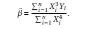
Take the linear model Y Æ X¯Åe with E[e j X] Æ 0 and X 2 R. Consider the estimatorFind the asymptotic distribution of p n ¡ b¯¡¯¢as n!1. . i=1
Take themodel Y Æ X1¯1 ÅX2¯2 Åe E[Xe] Æ 0 with both ¯1 2 R and ¯2 2 R, and define the parameter µ Æ ¯1¯2.(a) What is the appropriate estimator bµ for µ?(b) Find the asymptotic distribution of bµ under standard regularity conditions.(c) Show how to calculate an asymptotic 95%
Consider an i.i.d. sample {Yi ,Xi } i Æ 1, ...,n where Y and X are scalar. Consider the reverse projection model X Æ Y °Åu with E[Y u] Æ 0 and define the parameter of interest as µ Æ 1/°.(a) Propose an estimator b° of °.(b) Propose an estimator bµ of µ.(c) Find the asymptotic
Consider the modelwith both Y and X scalar. Assuming ® È 0 and ¯ Ç 0 suppose the parameter of interest is the area under the regression curve (e.g. consumer surplus), which is A Æ ¡®2/2¯.Let bµ Æ (b®, b¯)0 be the least squares estimators of µ Æ (®,¯)0 so that p n ¡bµ¡µ¢!d N(0,V
Take a regression model with i.i.d. observations (Yi ,Xi ) with X 2 RLet b¯ be the OLS estimator of ¯ with residuals bei Æ Yi ¡Xi b¯. Consider the estimators of (a) Find the asymptotic distribution of p n ¡e¡¢as n!1.(b) Find the asymptotic distribution of p n ¡b¡¢as n!1.(c) How
In the homoskedastic regression model Y Æ X0¯Åe with E[e j x] Æ 0 and E£e2 j X¤Æ ¾2 suppose b¯ is the OLS estimator of ¯ with covariance matrix estimator bV b¯ based on a sample of size n. Let b¾2 be the estimator of ¾2. You wish to forecast an out-of-sample value of YnÅ1 given that
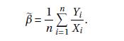
The model is Y Æ X¯Åe with E[e j X] Æ 0 and X 2 R. Consider the two estimators(a) Under the stated assumptions are both estimators consistent for ¯?(b) Are there conditions under which either estimator is efficient? B= B= Xi Yi 1 Yi n Y Xi
Find the asymptotic distribution of pn¡b¾2 ¡¾2¢as n!1.
Of the variables (Y ¤,Y ,X) only the pair (Y ,X) are observed. In this case we say that Y ¤ is a latent variable. Supposewhere u is a measurement error satisfyingLet b¯ denote the OLS coefficient fromthe regression of Y on X.(a) Is ¯ the coefficient fromthe linear projection of Y on X?(b) Is
The model isFind the method of moments estimators ( b¯,b) for ¡¯,¢. Y = X'+e E[Xe]=0 Q=E[XX' e].
Show (7.13)-(7.16).
Verify some of the calculations reported in Section 7.4. Specifically, suppose that X1 and X2 only take the values {¡1,Å1}, symmetrically, withVerify the following: PIX1 X2=1]=P[X = X2=-1] = 3/8 PIX =1,X2=-1]P[X =-1, X2 = 1] = 1/8 E [e | X = X2] = Ee XX2] = 5 4 4
For the ridge regression estimator (7.43), set ¸ Æ cn where c È 0 is fixed as n !1. Find the probability limit of b¯ as n!1.
Take themodel Y Æ X0¯Åe with E[Xe] Æ 0. Define the ridge regression estimatorhere ¸ È 0 is a fixed constant. Find the probability limit of b¯ as n!1. Is b¯ consistent for ¯? n B=XiX+MIK i=1 n i=1 (7.43)
Take themodel Y Æ X0 1¯1ÅX0 2¯2Åe with E[Xe] Æ 0. Suppose that ¯1 is estimated by regressing Y on X1 only. Find the probability limit of this estimator. In general, is it consistent for ¯1? If not, under what conditions is this estimator consistent for ¯1?
In the normal regression model let s2 be the unbiased estimator of the error variance ¾2 from (4.31).(a) Show that var£s2¤Æ 2¾4/(n ¡k).(b) Show that var£s2¤is strictly larger than the Cramér-Rao Lower Bound for ¾2.
Show (5.20).
Show that the test “Reject H0 if LR ¸ c1” for LR defined in (5.18), and the test “Reject H0 if F ¸ c2” for F defined in (5.19), yield the same decisions if c2 Æ¡exp(c1/n)¡1¢(n ¡k)/q. Does this mean that the two tests are equivalent?
Let b C¯ Æ [L,U] be a 1¡® confidence interval for ¯, and consider the transformation µ Æ g (¯)where g (¢) is monotonically increasing. Consider the confidence interval b Cµ Æ [g (L), g (U)] for µ. Show that P£µ 2 b Cµ¤Æ P£¯ 2 b C¯¤. Use this result to develop a confidence
Let F(u) be the distribution function of a random variable X whose density is symmetric about zero. (This includes the standard normal and the student t .) Show that F(¡u) Æ 1¡F(u).
In the normal regression model show that the robust covariance matrices bV HC0 b¯ , bV HC1 b¯ , bV HC2 b¯ , and bV HC3 b¯ are independent of the OLS estimator b¯, conditional on X .
In the normal regression model show that the leave-one out prediction errors eei and the standardized residuals ei are independent of b¯, conditional on X .Hint: Use (3.45) and (4.29).
For the regression in-sample predicted values b Yi show that b Yi j X » N¡X0 i¯,¾2hi i¢where hi i are the leverage values (3.40).
Show that argmaxµ2£ `n(µ) Æ argmaxµ2£ Ln(µ).
Show that if e »N(0,§) and § Æ AA0 then u Æ A¡1e »N(0, I n) .
Show that if e »N¡0, I n¾2¢and H0H Æ I n then u Æ H0e »N¡0, I n¾2¢.
Show that if Q » Â2r, then E[Q] Æ r and var[Q] Æ 2r.Hint: Use the representation Q ÆPniÆ1 Z2 i with Zi independent N(0,1) .
Extend the empirical analysis reported in Section 4.21 using the DDK2011 dataset on the textbook website.. Do a regression of standardized test score (totalscore normalized to have zero mean and variance 1) on tracking, age, gender, being assigned to the contract teacher, and student’s percentile
Continue the empirical analysis in Exercise 3.26. Calculate standard errors using the HC3 method. Repeat in your second programming language. Are they identical?
Continue the empirical analysis in Exercise 3.24.(a) Calculate standard errors using the homoskedasticity formula and using the four covariance matrices from Section 4.14.(b) Repeat in a second programming language. Are they identical?
Take the linear regression model with E[Y j X ] Æ X ¯. Define the ridge regression estimator b¯ Æ¡X 0X ÅI k¸¢¡1 X 0Y where ¸ È 0 is a fixed constant. Find E£ b¯ j X¤. Is b¯ biased for ¯?
An economist friend tells you that the assumption that the observations (Yi ,Xi ) are i.i.d.implies that the regression Y Æ X0¯Åe is homoskedastic. Do you agree with your friend? How would you explain your position?
Showing 1500 - 1600
of 4105
First
9
10
11
12
13
14
15
16
17
18
19
20
21
22
23
Last
Step by Step Answers