New Semester Started Get 50% OFF Study Help! --h --m --s Claim Now

Question Answers

Textbooks

Find textbooks, questions and answers

Oops, something went wrong!

Change your search query and then try again

Result Not Found

Books FREE
Study Help
Tutors
AI Study Planner NEW
Sell Books

Search
Sign In
Register

study help
business
statistical sampling to auditing

Statistical Methods For The Social Sciences 3rd Edition Alan Agresti, Barbara Finlay - Solutions

5 Table 11 11 show's a SAS printout from fitting the multiple regression model to the data hom Table 9.1. excluding D.C., on Y = violent crime rate. X = poverty rate. and X2 = pescent living in metropolitan areas TABLE 11.11 Sum of Mean Source DF Squares Model 2 2448368.07 Square 1224184.04 F Value
6. Repeat the previous exercise using software to fit the model with murder rate in Table 9.1 as the response variable.
7 Refer to Problem 11.5. With X3 = percentage of single-parent families also in the model. Table 11.12 shows results.a) Report the prediction equation and interpret the coefficientsb) Report R, and interpretc) Report the test statistic for Ho P ==B3 = 0. find its df values and P-value, and
8. Table 11.13 is part of a SPSS printout for fitting a regression model to the relationship between Y = number of children in family. X = mother's educational level (MEDUC) in years, and X2 father's socioeconomic status (FSES), for a random sample of 49 college students at Texas A&M University.a)
9 Refer to Problem 9.30 on feelings toward liberals, political ideology, and religious atten- dance. The sample size is small, but for illustrative purposes Table 11.14 shows results of fitting the inultiple regression model with feelings toward liberals as the response, using the category numbers
1 Studies of the degree of residential segregation between blacks and whites use the segre. gation index, defined as the percentage of nonwhites who would have to change the block on which they live in order to produce a fully nonsegregated city-one in which the per- centage of nonwhites living in
2. Refer to the previous exercise.a) State the assumptions for the analysis, and show that at least two of them may be vio- lated. What is the impact?b) Construct the regression model with dummy variables that applies for this ANOVA What does the estimate of the coefficient of Z equal?
3. A consumer protection group compares three different types of front bumpers for a bi and of automobile A test is conducted by driving an automobile into a brick wall at 15 mules per hour. The response is the amount of damage to the car, as measured by the repair costs, in hundreds of dollars Due
4. Table 1227 show's scores on the first quiz (maximum score 10 points) in a beginning French course. Students in the course are grouped as follows: Group A. Never studied foreign language before, but have good English skills Group B: Never studied loreign language before have poor English skills
5. The General Social Survey asks respondents to rate various groups using the "feeling ther- mometer Ratings between 50 and 100 mean you feel favorable and warm toward the group, whereas ratings between 0 and 50 mean that you don't feel favorable. When asked to rate liberals, the mean response was
6. Refer to Table 12.19.a) Using software, conduct a one-way ANOVA for the 72 observations at time = after. Verify that the F test statistic companng the three treatments at that time equals 8 65, based on df = 2 and df = 69, for which P = .0004.b) Show how to obtain the same results by conducting
7. Table 12 29 is a contingency table summarizing responses on political ideology in the 1991 General Social Survey by race and gender. Table 12.30 shows results of using SAS software to conduct an analysis of variance comparing the four groups, using the category labels for the ideology scores.a)
8. Refer to the previous exercise, using the black sample onlya) Conduct an ANOVA comparing the two groups. Interpret.b) How does your analysis relate to the methods of Chapter 7 for comparing means?c) How, if at all. would the results differ if you used ideology scores (i) (-3, -2, -1, 0. 1, 2,
9 Use software with the data in Table 9.4a) Conduct au ANOVA to test equality of the mean selling prices for homes with one. Two, and three bathrooms. Interpret.b) Explain the difference between conducting a test of independence of selling price and number of bathroonis using the ANOVA test in (a)
10. Refer to Table 9.4 In that data set, whether a house is new is a dummy variable Using software, put this as the sole predictor of selling price in a regression analysis.a) Conduct the test for the effect of this variable in the regression analysis (i.e., test Ho B=0). Interpretb) Conduct the F
11. A psychologist compares the mean amount of time of REM sleep for subjects under three conditions. She uses three groups of subjects, with four subjects in each group. Table 12.31 shows a SAS printout for the analysis.a) Report and interpret all steps of the ANOVA F test.b) Explain how to obtain
12. For g groups with large sample sizes, we plan to compare sinultaneously all pairs of popu- lation means. We want the probability to equal at least 80 that the entire set of confidence intervals contain the true differences.a) If g 10, which tabled t-score should we use for each interval?b)
13. A geographer compares residential lot sizes in four quadrants of a city To do this, he randomly samples 300 records from a city file on home residences and records the lot sizes (in thousands of square feet) by quadrant. The ANOVA table (Table 12.32) refers to a comparison of mean lot sizes for
14. A study compares the inean level of contributions to political campaigns in Pennsylvania by registered Democrats, registered Republicans, and unaffiliated votersa) Write a regression equation for this analysis, and interpret the parameters in the inodel.b) Explain how one can use the regression
15. Use computer software to reproduce the one-way ANOVA results reported in Table 12.2 for Example 12 1.
16. According to the US Department of Labor, the mean hourly wage in 1994 was $15.71 for a college graduate and $9.92 for a high school graduate. In 1979, the means (in 1994 dollars) were $15.52 for college graduates and $11.23 for high school graduates.a) Construct a 2x2 table to display the
17. Refer to Table 7.18 in Problem 7.40, which summanzes the mean number of dates in the past three months by gender and hy level of physical atu activeness. Do these data appear to show interaction? Explain.
18 A recent regression analysis of college faculty salaries in 1984 (M. Bellas, American So ciological Review. Vol. 59, 1994, p. 807) included a large number of predictors, including a dummy variable for gender (male = 1) and a dummy variable for race (nonwhite = 1) For annual income measured in
19. Refer to the prediction equation = 4 58.71P-54P-08G for the no interaction model in Example 12.5.a) Using it. find the estimated means for each of the six cells, and show that they satisfy a lack of interaction.b) Using results for this model, construct and interpret 95% Bonferroni confidence
20 Use software with Table 12.11, analyzed in Section 12.5.a) Fit the no interaction model, and verify the results given there.b) Fit the interaction model. Compare SSE for this model to SSE for the no interaction nodel. Show how the difference betw cen these values relates to the partial sum of
21. Consider the regression model E(Y) = a + BG + BR+B(GR), where Y = income (thousands of dollars), G= gender (G=1 for men and G = 0 for women), and R = race (R=1 for whites and R == 0 for blacks).a) Suppose that, in the population. B = 0. Interpret B, and 5b) The prediction equation for a certain
22. Refer to Problem 12.7. Table 12.33 shows the result of using SAS to conduct a two-way ANOVA, with both gender and race as predictors. The first panel of the table shows the result of the model with an interaction term, and the other three panels show results after dropping that term.a) Test the
23. Table 12 34 shows results of an ANOVA on Y = depression index and the predictors gen- der and marital status (married, never married. divorced).a) State the regression model for this analysis.b) State the sample size and fill in the blanks in the ANOVA tablec) Interpret the result of the F test
24. The 25 women faculty in the humanities division of a college have a mean salary of $46,000, whereas the five in the science division have a mean salary of $60,000. On the TABLE 12.34 Suni of Source Mean Squares DF Square F Prob F Gender 100 Marital status 200 Interaction 100 - 4000 205 Total
25 Refer to Example 12.6 and Table 12.16.a) Using software, conduct the repeated measures analyses of Section 12.6b) Suppose one scored the influence categones (1,2. 3. 4. 5). Would this have any effect on the test statistic" Explainc) Suppose one used scores (-3.-2 0, 2, 3). What would this assume
26. Recently the General Social Survey asked respondents. "Compared with ten years ago. would you say that American children today arc (1) much better off, (2) better off, (3) about the same. (4) worse off, oi (5) much worse off" Table 12.35 shows responses for ten of the subjects on three issues:
27 Refer to the previous exercise. The first five respondents were female, and the last five were male. Analyze these data using both gender and issue as factors.a) Identify the between-subjects and within-subjects factors.b) Test for interaction. Interpret.c) Test the main effect of gender.
28. Refer to Problem 125 When these subjects were asked to rate conservatives. the mean responses were 61.9 during 1983-87 and 60.7 during 1988-91. Explain why a two-way ANOVA using time (1983-87. 1988-91) and group rated (Liberal, Conservative) as fac- tors would require methods for repeated
29. Upjohn, a pharmaceutical company, conducted a randomized clinical tnal comparing an active hypnotic drug with a placebo for patients suffering from insomnia. The outcome is patient response to the question, "How quickly did you fall asleep after going to bed?" Patients suffering froin insomnia
30 Table 12.37 shows results of irsing SPSS in Example 12.7 with Table 12 19a) Explain how to use the information in this table to conduct the test of no interaction between treatment and time.b) Explain how to determine the df values for treatment. time, and their interaction.
31. Using software, conduct the repeated measures ANOVA in Example 12.7 with Table 12.19. Concepts and Applications
32. Refer to the WWW data sei (Problem 1.7). with response variable the number of weekly hours engaged in sports and other physical exercise. Using software, conduct an analysis of variance and follow-up estimation, and prepare a report summarizing your analyses and interpretations usinga) Gender
33 Refer to the data file created in Problems 1.7 For variables chosen by your instructor. use ANOVA methods and related inferential statistical analyses. Interpret and summarize your findings.
34. The General Social Survey has frequently asked respondents how they would rate van- ous countries on a scale from -5 to +5, where -5 indicates the country is disliked very much and +5 indicates the country is liked very much. Table 12.38 shows counts of the responses regarding ratings of Russia
35. A random sample of 26 female students at a major university were surveyed about their attitudes toward abortion. Each received a score on abortion attitude according to how many from a list of eight possible reasons for abortion she would accept as a legitimate reason for a woman to seek
36. Table 12.40, based on data from the 1989 General Social Survey, is a contingency table summarizing responses of 29 subjects regarding government spending on the environ-ment, assistance to big cities, and law enforcement The response scale was 1 too little, 2 = about right, 3 = too much.
37. Refer to the WWW data set in Problem 1.7. Use repeated measures analyses to model the weekly number of hours of recreation in terms of type of activity (levels S = sports and physical exercise, T = TV watching) and gender Interpret results of all analyses. and summanze.
38. An experiment used four randomly selected groups of five individuals each. The overall sample mean was 60.a) What did the data look like if the one-way ANOVA for comparing the means had test statistic F = 0?b) What did the data look like if F = 00?
39. Explain carefully the difference between a probability of Type I error of .05 for a single comparison of two means and a multiple comparison error rate of 05 for comparing all pairs of means
40 In multiple compansons following a one-way ANOVA, is it possible that group A is not significantly different from group B and group B is not significantly different from group C yet group A is significantly different from group C? Explain.
41. Construct a numerical example of means for a two-way classification under the following conditions:a) Main effects are present only for the row vanable.b) Main effects are present for each variable, but there is no interaction.c) Interaction effects are present.d) No effects of any type are
42. The null hypothesis of cquality of means for a factor is rejected in a two-way ANOVA Does this unply that the hypothesis will be rejected in a one-way ANOVA F test. if the data are collapsed over the levels of the second vanable? Explain.
43. For a two-way classification of means by factors A and B. at each level of B the means are equal for the levels of A. Docs this imply that the overall means are equal at the vari- ous levels of A. ignoring B" Explain the implications, in terms of how results may differ between two-way ANOVA and
44. Analysis of variance and regression are similar in the sense thata) They both assume a quantitative response variableb) They both have F tests for testing that the response variable is statistically independent of the explanatory variable(s)c) For inferential purposes, they both assume that the
45. Onc-way ANOVA provides relatively more evidence that Ho: 1 ==, is falsea) The smaller the "between" vanation and the larger the "within" variation.b) The smaller the "between" variation and the smaller the "within variation.c) The larger the "between" variation and the smaller the "within"
46. For four means. a multiple comparison method provides simultaneous 95% confidence intervals for the differences between the six pairs. Thena) For each confidence interval. there is a .95 chance that it contains the truc difference.b) The probability that all six confidence intervals are correct
47. Interaction tenns are needed in a two-way ANOVA model whena) Each pain of variables is associated.b) Both explanatory variables have significant effects in the model without interaction termsc) The difference in means between two categories of one explanatory variable varics greatly among the
48. * You know the sample mean, standard deviation, and sample size for each of three groups. Can you conduct an ANOVA F test. or would you need more information?
49 You form a 95% confidence interval in five different situations.a) Assuming that the results of the intervals are statistically independent. find the proba- bility that all five intervals contain the parameters they are designed to estimate. Find the probability that at least one interval is in
50 * Show how to construct a regression model for the analysis of mean income over a three- way classification of gender (male, female). race (white, black), and type of job (assembly- line worker. janitorial). Interpret the parameters in the model. Assume that there is no interaction
51. *This exercise motivates the formula for the between estimate of the variance in one-way ANOVA. Suppose the sample sizes all equal n and the population means all equal . The sampling distribution of each Y, then has mean and vanance o/n. The sample mean of the values, when the sample sizes are
52. The Scheffe multiple comparison method for comparing g groups with overall error rate a provides interval for -; of - + where F denotes the value from the F distribution with df = g-1 and dj = N-g having right-tail probabilitya. Apply this method to Example 12.3. interpret results, and compare
1. The regression equation relating education (number of years completed) to race (Z = 1 for whates. Z = 0 foi nonwhites) in a certain country is E(Y) = 11+2Z. The regression equation relating education to race and to father's education (X) is E(Y)=3+.8X-.6Z.a) Find the mean education for whites.
2 A regression analysis for the 100th Congress, ending in 1988, predicted the proportion of each representative's votes on abortion issues that took the "pro-choice" position (R. Tatalovich and D. Schier. American Politics Quarterly. Vol. 21, 1993, p. 1251. The pre- diction equation was =.350 +
3. Based on a national survey Table 13.14 shows results of a prediction equation (ignoring some nonsignificant vanables) reported for the response variable. Y = alcohol consump- tion, measured as the number of alcoholic drinks the subject drank during the past month (D. Umberson and M Chen,
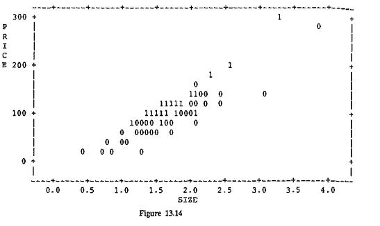
4. Refer to Table 9.4 in Chapter 9 Table 13.15 shows a printout for modeling Y = selling price in terms of X = size of home and Z = whether the home is new (Z = 1. yes; Z= 0), no).
5 Refer to the previous exercise Table 13.16 shows a SPSS printout from fitting the model allowing interaction. where NEWSIZE refers to the cross-product term. TABLE 13.16 R Square Adjusted R Square .8675 .8630 Standard Error 16.3509 Analysis of Variance DF Sum of Squares Regression 3 155811.60588
6 Refer to the previous problem. Figure 13.14 shows a SAS scatter diagram for the rela- tionship between selling price and size of home. identifying the points by a 1 when the home is new and a 0 when it is not. Because of the crudeness of scale, many of the points are hidden in this plot, but note
7 Refer to Table 13 1. Not reported there were observations for ten Asian Americans. Their (X, Y) values follow: Subject Education 16 14 2 3 4 5 12 18 Income 35 21 36 13 12 28 16 19 29 629 7 8 9 10 16 16 14 10 41 18 10a) Fit the analysis of covariance model using all four groups, assuming no
8. The printouts in Table 13.18 show results of using SAS to fit four models to data from a study of the relationship between Ypercentage of adults voting, X = percentage of adults registered to vote. and racial-ethnic representation, for precincts in the state of Texas for a gubernatorial election
9. Refer to the previous exercise The means of percentage registered for the three categories are X = 762, X = 49.5. ;= 39.7, with an overall mean of X = 60.4a) Find the adjusted means on percentage voting, and interpret.b) Compare the adjusted mean for Auglos to the unadjusted mean of 52 3, and
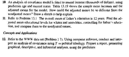
10 An analysis of covariance model is fitted to annual income (thousands of dollars), using predictors age and mantal status Table 13.19 shows the sample mean incomes and the adjusted means for the model. How could the adjusted means be so different from the unadjusted means Draw a sketch to help
11. Refer to Problem 13.1 The overall mean of father's education is 12 years Find the ad- justed mean educational levels for whites and nonwhites, controlling for father's educa- tion, and compare them to the unadjusted means. Concepts and Applications
12. Refer to the WWW data set (Problem 17). Using computer software, conduct and inter- pret an analysis of covariance using Y = political ideology. Prepare a report, presenting graphical, descriptive, and inferential analyses. using the predictors TABLE 13.19 Mcan Mean Adjusted Mean Group Age
13 Repeat the previous excrcise. using = college GPA with predictors high school GPA. gender, and religiosity.
14. Refer to the data file created in Problem 1.7. For variables chosen by your instructor. use regression analysis as the basis of descnptive and inferential statistical analyses Sun- marize your findings in a report in which you describe and interpret the fitted models and the related analyses
15 Table 13.20 shows results of fitting a regression model to data from 1969 on salaries (in dollars) of about 35.000 college professors. Four predictors are qualitative (binary), with dummy vanable defined in parentheses The table shows estimates of parameters for each predictor, with standard
16. * Table 13 21 is a SPSS printout based on General Social Survey data combined for the years 1977, 1978, and 1980. The response vanable is an index of attitudes toward pre- marital. extramarital, and homosexual sex. Higher scores represent more permissive atti-tudes. The qualitative explanatory
17. A researcher is interested in factors associated with fertility in a Latin American city. Of particular interest is whether migrants from other cities or migrants from rural areas differ from natives of the city in their completed family sizes. The groups to be compared are urban natives, urban
18. Refer to Table 91, not including the observation for DC. Let Z be a dummy variable for whether a state is in the South. with Z=1 for AL. AR. FL. GA KY, LA, MD, MS, NC, OK, SC, TN, TX, VA, WVa) Analyze the relationship between Y = violent crime rate and the predictors X = poverty rate and Z.b)
19. Refer to the previous exercise. Repeat using Y = murder late 20. Figure 13 4 exhibits at least one possibly influential outlier Remove the observation with the highest income and reconduct the analyses. Did this one observation have any influ- ence on the results?
21. You have two groups, and you want to compare their regressions of Y on X, in order to test the hypothesis that the true slopes are identical for the two groups. Explain how you can do diis using regression modeling.
22 Le Y = death rate and X = average age of residents. measured for each county in Mas- sachusetts and in Florida. Draw a hypothetical scatter diagrain, identifying points for each state, whena) The mean death rate is higher in Florida than in Massachusetts when X is ignored, but lower when it is
23. Draw a scatter diagram of X and Y with sets of points representing two groups such that Ho equal means on Y would be rejected in a one-way ANOVA. but would not be rejected in an analysis of covariance.
24. Give an example of a situation in which you expect interaction between a quantitative variable and a qualitative variable in their effects on a quantitative response variable. In Problems 13.25-13.26, select the correct response(s)
25 In the model E(Y) =+P,X+BZ. where Z is a dummy variable,a) The qualitative predictor has two categories.b) One line has slope B, and the other has slope .c) is the difference between the mean of Y for the second and first categories of the qualitative variable.d) is the difference between the
26 In the United States, the mean annual income for blacks (4) is smaller than for whites (2). the mean number of years of education is smaller for blacks than for whites, and annual income is positively related to number of years of education. Assuming that there is no interaction, the difference
27. Summarize the differences in purpose of the following:a) A regression analysis for two quantitative vanablesb) A one-way analysis of variancec) A two-way analysis of vananced) An analysis of covariance
1 Refer to Table 9.1, deleting the observation for DC With Y = violent crime rate and the five predictors as explanatory variables (all except murder rate) and using a = 10 in tests, select a model using (a) backward elimination. (b) for ward selection. Jinterpret the model selected.
2. Refer to Table 9.1, excluding the observation for DC Let predictors in that table (excluding violent crime rate), the bivariate model has P-value below 05 = muider rate. For the five test of independence for thea) Fit the multiple regression model, using all five predictors. Are the P-values for
3. Refer to the previous problem Now include the DC observationa) Use backward elimination. and compare results to part (b) above.b) Use forward selection, and compare results to part (c) above.c) What does this exercise suggest about how influential outliers can be on the results of automatic
4. Refer to Problem 14 2(b) Use backward elimination again with the variables chosen in (b) and their interactions Does the resulting model make sense?
5 Refer to Example 11.2 on Y = mental impairment. X = life events. and X = SES.a) Show that forward selection with X. X. X = XX. XX. and X, = X and the a=.10 level for inchision selects only X1 and X2 for the model.b) Use backward climination. What is the final model? Interpretc) Use the C, index
6. Use backward elimination with the home sales data of Table 94, using as candidates the four explanatory variables and all their interaction and quadratic (square) terms What model do you end up with? Is this a reasonable model? Explain
7. Problem 13.6 showed that for the home sales data, a single observation has a large im pact on whether an interaction term seems needed in the model. Let's check whether that observation affects results of selection procedures Using regression software after delet- ing that observation from the
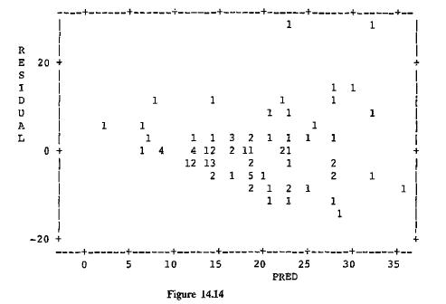
8. Figure 14.14 is a SAS plot of the residuals versus the predicted values for the analysis of covariance model discussed in Example 13.1 relating income to education and racial- ethnic group. What does this plot suggest? E 20+ RESIDUAL 0 -+------+------+------+------+---- -+-- 1 1 1 1 1 1 1 1 1 1
9. Refer to the model for housing price selected in Example 14.1.a) Study the studentized residuals, and show that only one is unusually large. What does this reflect?b) Study the hat values. Which three observations have the greatest leverage. and hence the predictor values with the greatest
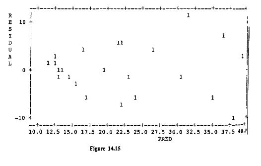
10. Refer to Problem 9 17 and Table 9 13. Table 14.8 shows a SAS computer printout of var- ious diagnostics from filling the muluple regression model relating birth rate to literacy and women's economic activity (deleung Germany. South Africa. and Vietnam). Figure 14 15 plots the residuals against
11. Based on the answers in the previous exercise. remove an observation that seems poten- tially influential to you, and re-fit the model. Is the new fit different in any substantive way?
12 Refer to Table 9.1. and fit the linear regression model relating = violent crime rate to Xpercent metropolitan for all 51 observationsa) Find the prediction equation. Using a stem and leaf plot or a histogram, plot the resid- uals. Interpret.b) Plot the residuals against the predictor
13. Refer to the previous exercise, and use software to obtain regression diagnosticsa) Study the studentized residuals. Are there any clear outliers?b) Study the liat values. Are there any observations with noticeable leverage?c) Based on the answers in (a) and (b). docs it seem as if any
14 Refer to Example 11 1. Fit the multiple regression model discussed there. for the data from Problem 9.24 Plot the residuals against each predictor and/or against the predicted values Do the plots show any irregularities?
15. Refer to Table 9.1. Let violent crime rate. Fit the model to the 51 observations with percentage in poverty and percentage of single-parent families as predictors.a) Report the prediction equation.b) Construct a stem and leaf plot or a histogram of the residuals. Interpret.c) Plot the residuals
16 Refer to the previous exercise. and use software to obtain regression diagnosticsa) Based on hat values and studentized esiduals, does it seem as if any observations may be influential? Explain.b) Study the DFFITS values Which, if any, observations have a strong influence on the fitted values?c)
17. This problem shows that multicollinearity also affects precision of estimation of partial correlations.a) Suppose the true correlations are px,x = .85, prx, = .65. and pix; = .65. Show that pyx, x- Prx; x = .244.b) In a sample. x, x = .9. ryx = .7 and Frx, = .6. Unless the sample is very large,

Showing 3400 - 3500 of 4976

First
28
29
30
31
32
33
34
35
36
37
38
39
40
41
42
Last

Step by Step Answers

Services

Sitemap
Fun
Definitions
Become Tutor
Used Textbooks
Study Help Categories
Recent Questions
Expert Questions
Campus Wear
Sell Your Books

Company Info

Security
Copyrights
Privacy Policy
Terms & Conditions
SolutionInn Fee
Scholarship
Online Quiz
Give Feedback, Get Rewards

Get In Touch

About Us
Contact Us
Career
Jobs
FAQ
Student Discount
Campus Ambassador

Secure Payment

Download Our App

© 2026 SolutionInn. All Rights Reserved