Questions and Answers of Systems Analysis And Design

Software does not break or wear out with time (unlike hardware). Why does software fail even after a good amount of testing?
What is the tester’s role in software development?
When to stop testing is a very crucial decision. What factors should be considered for taking such a decision?
Differentiate between(i) Alpha and Beta testing(ii) Development and regression testing(iii) Fault, bug and failure(iv) Verification and validation(v) Static and dynamic testing(vi) Program and
Explain a typical test case template. What are the reasons for documenting test cases?
With the help of a suitable example, illustrate why exhaustive testing is not possible.
Define a test case. What are the objectives of test case design? Discuss the various steps involved.
What is the role of Quality Assurance in software development? How is it different from Quality Control?
What is software crisis? Was Y2K a software crisis?
What are the components of a software system? Discuss how a software differs from a program.
Differentiate between generic and customized software products. Which one has a large market share and why?
What is a software failure? Discuss the conditions of a failure. Mere presence of faults may not lead to failures. Explain with the help of an example.
Verification and validation are used interchangeably many times. Define these terms and establish their relationship with testing.
Testing is not a single phase in the software development life cycle. Explain and comment.
Discuss the advantages of testing with reference to the software product.
Discuss the significance of the V-shaped software life cycle model and also establish the relationship between its development and testing parts.
What is the relationship of the V-shaped software life cycle model with the waterfall model? How is acceptance testing related to requirement analysis and specification phase?
Differentiate between the V-shaped software life cycle model and the waterfall model.
What is functional testing?(f) Test cases are designed on the basis of internal structure of the source code.(g) Test cases are designed on the basis of functionality, and internal structure of the
Which of the following statement is correct?(a) Functional testing is useful in every phase of the software development life cycle.(b) Functional testing is more useful than static testing because
Which of the following is not a form of functional testing?(a) Boundary value analysis(b) Equivalence class testing(c) Data flow testing(d) Decision table based testing
Functional testing is known as:(a) Regression Testing(b) Load Testing(c) Behaviour Testing(d) Structural Testing
For a function of ‘n’ variables, boundary value analysis generates:(a) 8n + 1 test cases(b) 6n + 1 test cases(c) 2n + 1 test cases(d) 4n + 1 test cases
For a function of 4 variables, boundary value analysis generates:(a) 9 test cases(b) 17 test cases(c) 33 test cases(d) 25 test cases
For a function of ‘n’ variables, robustness testing yields:(a) 6n + 1 test cases(b) 8n+ 1 test cases(c) 2n + 1 test cases(d) 4n + 1 test cases
For a function of ‘n’ variables, worst case testing generates:(a) 6n test cases(b) 4n + 1 test cases(c) 5n test cases (d) 6n + 1 test cases
For a function of ‘n’ variables, robust worst case testing generates:(a) 4n test cases(b) 6n test cases(c) 5n test cases(d) 7n test cases
A software is designed to calculate taxes to be paid as per details given below:(i) Up to Rs. 40,000 : Tax free(ii) Next Rs. 15,000 : 10% tax(iii) Next Rs. 65,000 : 15% tax(iv) Above this amount :
‘x’ is an input to a program to calculate the square of the given number. The range for‘x’ is from 1 to 100. In boundary value analysis, which are valid inputs?(a) 1,2,50,100,101(b)
‘x’ is an input to a program to calculate the square of the given number. The range for‘x’ is from 1 to 100. In robustness testing, which are valid inputs?(a) 0, 1, 2, 50, 99, 100, 101(b) 0,
Functionality of a software is tested by:(a) White box testing(b) Black box testing(c) Regression testing(d) None of the above
One weakness of boundary value analysis is:(a) It is not effective(b) It does not explore combinations of inputs(c) It explores combinations of inputs(d) None of the above
Boundary value analysis technique is effective when inputs are:(a) Dependent(b) Independent(c) Boolean(d) None of the above
Equivalence class testing is related to:(a) Mutation testing(b) Data flow testing(c) Functional testing(d) Structural testing
In a room air-conditioner, when the temperature reaches 28oC, the cooling is switched on. When the temperature falls to below 20oC, the cooling is switched off. What is the minimum set of test input
If an input range is from 1 to 100, identify values from invalid equivalence classes.(a) 0, 101(b) 10, 101(c) 0, 10(d) None of the above
In an examination, the minimum passing marks is 50 out of 100 for each subject.Identify valid equivalence class values, if a student clears the examination of all three subjects.(a) 40, 60, 70(b) 38,
How many minimum test cases should be selected from an equivalence class?(a) 2(b) 3(c) 1(d) 4
Decision tables are used in situations where:(a) An action is initiated on the basis of a varying set of conditions(b) No action is required under a varying set of conditions(c) A number of actions
How many portions are available in a decision table?(a) 8(b) 2(c) 4(d) 1
How many minimum test cases are generated by a column of a decision table?(a) 0(b) 1(c) 2(d) 3
The decision table which uses only binary conditions is known as:(a) Limited entry decision table(b) Extended entry decision table(c) Advance decision table(d) None of the above
In cause-effect graphing technique, causes and effects are related to:(a) Outputs and inputs(b) Inputs and outputs(c) Sources and destinations(d) Destinations and sources
Cause-effect graphing is one form of:(a) Structural testing(b) Maintenance testing(c) Regression testing(d) Functional testing
Which is not a constraint applicable at the ‘causes’ side in the cause-effect graphing technique?(a) Exclusive(b) Inclusive(c) Masks(d) Requires
Which is not a basic notation used in a cause-effect graph?(a) NOT(b) OR(c) AND(d) NAND
Which is the term used for functional testing?(a) Black box testing(b) Behavioural testing(c) Functionality testing(d) All of the above
Functional testing does not involve:(a) Source code analysis(b) Black box testing techniques(c) Boundary value analysis(d) Robustness testing
What is functional testing? How do we perform it in limited time and with limited resources?
What are the various types of functional testing techniques? Discuss any one with the help of an example.
Explain the boundary value analysis technique with a suitable example.
Why do we undertake robustness testing? What are the additional benefits? Show additional test cases with the help of an example and justify the significance of these test cases.
What is worst-case testing? How is it different from boundary value analysis? List the advantages of using this technique.
Explain the usefulness of robust worst-case testing. Should we really opt for this technique and select a large number of test cases? Discuss its applicability and limitations.
Consider a program that determines the previous date. Its inputs are a triple of day, month and year with its values in the range:1 month 12 1 day 31 1850 year 2050 The possible outputs are
Consider the program to find the median of three numbers. Its input is a triple of positive integers (say x, y and z) and values are from interval [100,500]. Generate boundary, robust and worst-case
Consider a program that takes three numbers as input and print the values of these numbers in descending order. Its input is a triple of positive integers (say x, y and z)and values are from interval
Consider a three-input program to handle personal loans of a customer. Its input is a triple of positive integers (say principal, rate and term).1000 principal 40000 1 rate 18 1 term 6 The program
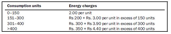
The BSE Electrical company charges its domestic consumers using the following slab:Identify the equivalence class test cases for output and input domain. Consumption units 0-150 151-300 301-400 >400
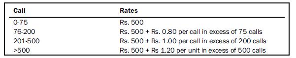
An telephone company charges its customer using the following calling rates:Identify the equivalence class test cases for the output and input domain. Call 0-75 76-200 201-500 >500 Rates Rs. 500 Rs.
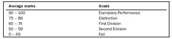
Consider an example of grading a student in a university. The grading is done as given below:The marks of any three subjects are considered for the calculation of average marks.Generate boundary
Consider a program for the classification of a triangle. Its input is a triple of positive integers (say,a, b andc) from the interval [1, 100]. The output may be one of the following words [scalene,
Consider a program that determines the next date. Given a month, day and year as input, it determines the date of the next day. The month, day and year have integer values subject to the following
Consider a program for the determination of the nature of roots of a quadratic equation.Its input is a triple of positive integers (saya, b andc) and values may be from interval[0, 100]. The output
Explain the equivalence class testing technique. How is it different from boundary value analysis technique?
Discuss the significance of decision tables in testing. What is the purpose of a rule count? Explain the concept with the help of an example.
What is the cause-effect graphing technique? What are basic notations used in a causeeffect graph? Why and how are constraints used in such a graph?
Consider a program to multiply and divide two numbers. The inputs may be two valid integers (say a andb) in the range of [0, 100].(a) Generate boundary value analysis test cases and robust test
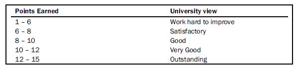
Consider the following points based on faculty appraisal and development system of a university:Generate the test cases using equivalence class testing. Points Earned 1-6 6-8 8-10 10-12 12-15
Consider a program to perform binary search and generate the test cases using equivalence class testing and decision table based testing.
Write a program to count the number of digits in a number. Its input is any number from interval [0, 9999]. Design the boundary value analysis test cases and robustness test cases.
Why is functional testing also known as black box testing? Discuss with the help of examples.
What are the limitations of boundary value analysis technique? Discuss the situations in which it is not effective.
Cyclomatic complexity is designed by:(a) T.J. McCabe(b) B.W. Boehm(c) Victor Basili(d) Bev. Littlewood
Cyclomatic complexity can be calculated by:(a) V(G)= e-n+2P(b) V(G)= +1(c) V(G)= number of regions of the graph(d) All of the above
The cyclomatic complexity equation V(G)= +1 is applicable only if every predicate node has:(a) Two outgoing edges(b) Three or more outgoing edges(c) No outgoing edge(d) One outgoing edge
Cyclomatic complexity is equal to:(a) Number of paths in a graph(b) Number of independent paths in a graph(c) Number of edges in a graph(d) Number of nodes in a graph
A node with indegree 0 and outdegree =0 is called:(a) Source node(b) Destination node(c) Predicate node(d) None of the above
A node with indegree =0 and outdegree 0 is called:(a) Source node(b) Destination node(c) Predicate node(d) Transfer node
An independent path is:(a) Any path that has at least one new set of processing statements or new condition(b) Any path that has at most one new set of processing statements or new condition(c) Any
DD path graph is called:(a) Defect to defect path graph(b) Design to defect path graph(c) Decision to decision path graph(d) Destination to decision path graph
Every node in the graph matrix is represented by:(a) One row and one column(b) Two rows and two columns(c) One row and two columns(d) Two rows and one column
The size of graph matrix is:(a) Number of edges in the flow graph(b) Number of nodes in the flow graph(c) Number of paths in the flow graph(d) Number of independent paths in the flow graph
A program with high cyclomatic complexity is:(a) Large in size(b) Small in size(c) Difficult to test(d) Easy to test
Developers may have to take some tough decisions when the cyclomatic complexity is:(a) 1(b) 5(c) 15(d) 75
Every node of a regular graph has:(a) Different degrees(b) Same degree(c) No degree(d) None of the above
The sum of entries of any column of incidence matrix is:(a) 2(b) 3(c) 1(d) 4
The sum of entries of any row of adjacency matrix gives:(a) Degree of a node(b) Paths in a graph(c) Connections in a graph(d) None of the above
The adjacency matrix of a directed graph:(a) May have diagonal entries equal to 1(b) May be symmetric(c) May not be symmetric(d) May be difficult to understand
Length of a path is equal to:(a) The number of edges in a graph(b) The number of nodes in a graph(c) The number of nodes in a path(d) The number of edges in a path
Strongly connected graph will always be:(a) Weakly connected(b) Large in size(c) Small in size(d) Loosely connected
A simple graph has:(a) Loops and parallel edges(b) No loop and a parallel edge(c) At least one loop(d) At most one loop
In a directed graph:(a) Edges are the un-ordered pairs of nodes(b) Edges are the ordered pairs of nodes(c) Edges and nodes are always equal(d) Edges and nodes are always same
What is a graph? Define a simple graph, multigraph and regular graph with examples.
How do we calculate degree of a node? What is the degree of an isolated node?
What is the degree of a node in a directed graph? Explain the significance of indegree and outdegree of a node.
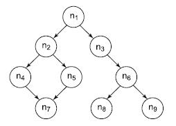
Consider the following graph and find the degree of every node. Is it a regular graph?Identify source nodes, destination nodes, sequential nodes, predicate nodes and junction nodes in this graph. 2
Consider the graph given in exercise
and find the following:(i) Incidence matrix(ii) Adjacency matrix(iii) Paths(iv) Connectedness(v) Cycles
Define incidence matrix and explain why the sum of entries of any column is always 2.What are various applications of incidence matrix in testing?

Showing 400 - 500 of 480