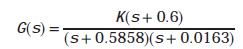
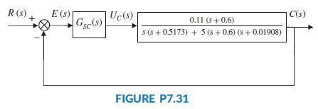
In Problem 71, Chapter 8, we used MATLAB to plot the root locus for the speed control of an HEV rearranged as a unity-feedback system, as shown in Figure P7.31 (Preitl, 2007). The plant and compensator were given by

and we found that K = 0.78, resulted in a critically damped system.

a. Use MATLAB or any other program to plot the following:

i. The Bode magnitude and phase plots for that system, and
ii. The response of the system, c(t), to a step input, r(t) = 4 u(t). Note on the c(t) curve the rise time, T_r, and settling time, T_s, as well as the final value of the output.

b. Now add an integral gain to the controller, such that the plant and compensator transfer function becomes

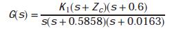
where K₁=0.78 and Zc = K/K₁ = 0.4. Use MATLAB or any other program to do the following:

i. Plot the Bode magnitude and phase plots for this case.
ii. Obtain the response of the system to a step input, r(t) = 4 u(t). Plot c(t) and note on it the rise time, T_r, percent overshoot, %OS, peak time, T_p, and settling time, T_s.

c. Does the response obtained in Parts a orbresembleasecond-order overdamped, critically damped, or underdamped response? Explain.

Transcribed Image Text:

K(s+ 0.6) G(s) = (s+ 0.5858)(s+ 0.0163)