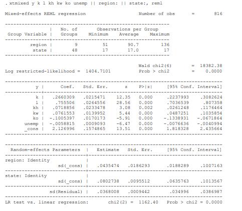
Using the Munnell (1990) data set considered in the empirical example, estimate the Cobb-Douglas production function investigating the productivity of public capital in each state's private output using nested MLE and REML as shown in the Stata output in Tables 9.5 and 9.6.

Table 9.5:

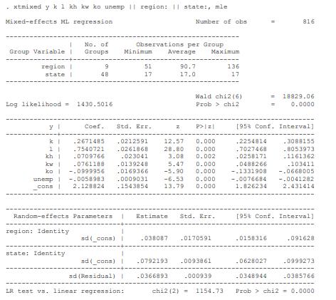
Table 9.6:

xtmixed y k 1 kh kw ko unemp region: | state:, mle Mixed-effects ML regression Number of obs 816 Group Variable No. of Groups Observations per Group Minimum Average Maximum region 9 51 90.7 state I 48 17 17.0 136 17 Log likelihood - 1430.5016 Wald chi2 (6) Prob > chi2 = 18829.06 0.0000 y l Coef. Std. Err. z P>|z [95% Conf. Interval] k | .2671485 .0212591 12.57 0.000 .2254814 .3088155 1.7540721 .0261868 28.80 0.000 .7027468 -8053973 kh 1.0709766 .023041 3.08 kw .0761188 .0139248 ko -.0999956 .0169366 unemp cons .0058983 2.128824 .0009031 .1543854 0.002 5.47 0.000 -5.90 -6.53 0.000 13.79 0.000 .0258171 .1161362 .0488266 .103411 0.000 -.1331908 -.0668005 -.0076684 -.0041282 1.826234 2.431414 Random-effects Parameters Estimate Std. Err. [95% Conf. Interval] region: Identity sd(_cons) .038087 .0170591 .0158316 .091628 state: Identity sd(_cons) | .0792193 .0093861 .0628027 .0999273 sd (Residual) .0366893 .000939 .0348944 .0385766 LR test vs. linear regression: chi2 (2) 1154.73 Prob chi2 0.0000