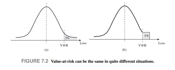
Consider the two loss densities in Fig. 7.2. In Fig. 7.2(a), we observe a normally distributed loss and its \(95 \%\) V @R, which is just its quantile at probability level 95\%; the area of the right tail is 5\%. In Fig. 7.2(b), we observe a sort of truncated distribution, obtained by replacing the tail of the normal PDF with a uniform density. The tail accounts for \(5 \%\) of the total probability. By construction, V \(@ \mathrm{R}\) is the same in both cases, since the areas of the right tails are identical. However, we might not associate the same risk with the two distributions. In the case of the normal distribution, there is no upper bound to loss; in the second case, there is a clearly defined worst-case loss. Whether the risk for density

(a) is larger than density

(b) or not, it depends on how we measure risk exactly; the point is that V@R cannot tell the difference between them.

Data From Figure 7.2

Transcribed Image Text:

5% Loss V@R (a) 5% Loss V@R (b) FIGURE 7.2 Value-at-risk can be the same in quite different situations.