

The covariance matrix for two correlated assets is whose inverse is Clearly, the inverse exists if we
Question:
The covariance matrix for two correlated assets is
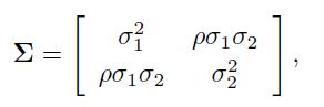
whose inverse is
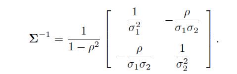
Clearly, the inverse exists if we rule out the case of perfect correlation \((=1)\). Then, the weights in the optimal portfolio are
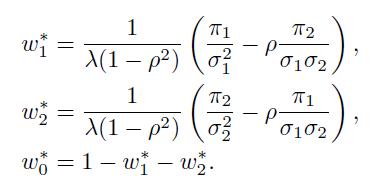
Note that, since we do not constrain the portfolio in any way, the weight of an asset can be positive or negative, depending on the sign and the size of the risk premia, on the volatilities, and on the correlation. For instance, let us rewrite the weight of asset 1 in terms of the Sharpe ratios 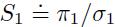 and
and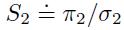 :
:
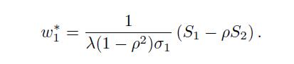
With a sufficiently large correlation, so that there is no diversification effect, if \(S_{2}\) is sufficiently larger than \(S_{1}\), we should sell the first asset short.
These expressions are useful to check the sensitivity of the portfolio composition to the input data and to challenge our intuition. What about the sensitivity to risk aversion? We see that
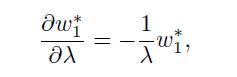
which may be positive or negative. If we hold a long (positive) position in the risky asset 1, increasing risk aversion will decrease its weight. However, if asset 1 is sold short, increasing will increase the portfolio weight, in the sense that it is shrunk towards zero (we reduce the amount of short-selling).
An easy finding is
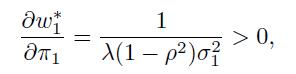
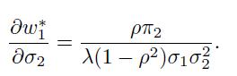
which makes good sense: The larger the risk premium of an asset, the larger the corresponding portfolio weight. One would expect that increasing the risk premium of the other asset will drive the portfolio weight down, which is not necessarily true. In fact,
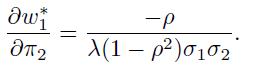
In the case of negative correlation, increasing 2 will increase both \(w_{1}\) and \(w_{2}\), because of a diversification effect. This effect is less strong when risk aversion and volatilities are large, and it is increasing with the absolute value of the correlation. By a similar token, the effect of increasing the volatility of the other asset depends on the sign of the correlation:
When correlation is positive, increasing the volatility of the second asset increases the weight of the first one, but the contrary applies with negative correlation.
The sensitivity of  with respect to
  is trickier:
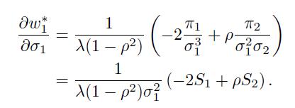
If the two Sharpe ratios are positive and close enough, this sensitivity will be negative, which corresponds to our intuition. However, the sensitivity can be positive. For instance, this may happen if risk premia are both positive, as well as correlation, but asset 1 has a smaller Sharpe ratio, so that it is sold short. An increase in volatility will increase its weight, in the sense that we should reduce the amount of short-selling in this case.
The analysis of sensitivity with respect to correlation is left as an exercise. We only observe that if risk premia are positive and we change a positive correlation into a negative one, without changing its absolute value, we will increase the exposure to both risky assets. This is clearly due to a diversification effect.
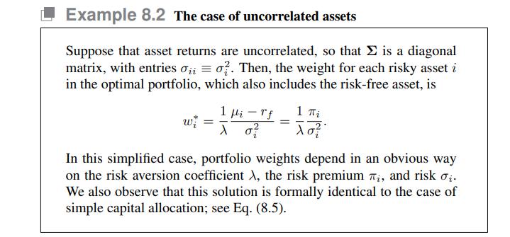
The bottom line of this example, with respect to the uncorrelated case of Example 8.2, is that introducing correlation makes the portfolio behavior less intuitive. In practice, we should also be aware that uncertainty in parameters may be interpreted as an effect of statistical estimation noise, which may have an adverse effect on the stability of the mean-variance optimal portfolio.
Data From Example 8.2
Data From Equation (8.5)
Step by Step Answer:


An Introduction To Financial Markets A Quantitative Approach
ISBN: 9781118014776
1st Edition
Authors: Paolo Brandimarte
