Consider Example 6.17 where the rice production function

was estimated using data from the file rice 5.

a. Using data from 1994 only, contrast the outcomes of the following hypothesis tests.

i. \(H_{0}: \beta_{2}=0\) versus \(H_{1}: \beta_{2} eq 0\), ii. \(H_{0}: \beta_{3}=0\) versus \(H_{1}: \beta_{3} eq 0\), iii. \(H_{0}: \beta_{2}=\beta_{3}=0\) versus \(H_{1}: \beta_{2} eq 0\) or \(\beta_{3} eq 0\) or both \(\beta_{2}\) and \(\beta_{3}\) are nonzero.

b. Show that the restricted model corresponding to the restriction \(\beta_{2}+\beta_{3}+\beta_{4}=1\) is given by

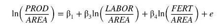
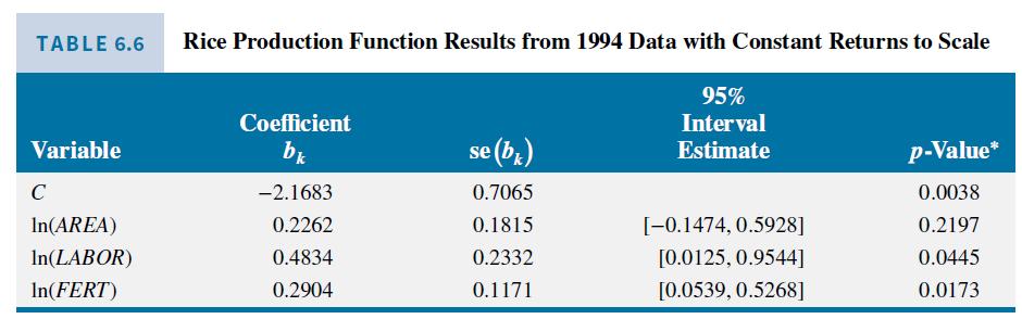
c. Some output from estimating the equation in part (b) using 1994 data is given in Table 6.6. It includes point and interval estimates for \(\beta_{2}, \operatorname{se}\left(b_{2}\right)\), and a \(p\)-value for testing \(H_{0}: \beta_{2}=0\) against \(H_{1}: \beta_{2} eq 0\). Describe how these results can be obtained and verify that they are correct.

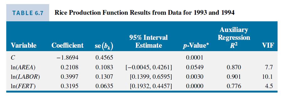
d. Estimate a constant-returns-to-scale production function using data from both 1993 and 1994. Compare the standard errors and \(95 \%\) interval estimates with those in Table 6.7 where both years of data were used, but constant returns to scale was not imposed. Include all coefficients in your comparison. What are the auxiliary \(R^{2}\) 's for the two variables in the restricted model?

Data From Example 6.17:-

To illustrate collinearity we use data on rice production from a cross section of Philippine rice farmers to estimate the production function

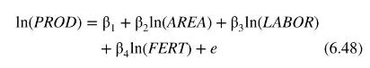
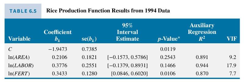
where PROD denotes tonnes of freshly threshed rice, \(A R E A\) denotes hectares planted, \(L A B O R\) denotes person-days of hired and family labor and FERT denotes kilograms of fertilizer. Data for the years 1993 and 1994 can be found in the file rice 5. One would expect collinearity may be an issue. Larger farms with more area are likely to use more labor and more fertilizer than smaller farms. The likelihood of a collinearity problem is confirmed by examining the results in Table 6.5, where we have estimated the function using data from 1994 only. These results convey very little information. The \(95 \%\) interval estimates are very wide, and, because the coefficients of \(\ln (A R E A)\) and \(\ln (L A B O R)\) are not significantly different from zero, their interval estimates include a negative range. The high auxiliary \(R^{2}\) 's and correspondingly high variance inflation factors point to collinearity as the culprit for the imprecise results. Further evidence is a relatively high \(R^{2}=0.875\) from estimating (6.48), and a \(p\)-value of 0.0021 for the joint test of the two insignificant coefficients, \(H_{0}: \beta_{2}=\beta_{3}=0\).

Data From Table 6.6 and 6.7:-

Transcribed Image Text:

In(PROD) B+ Bln(AREA) + 3ln(LABOR) + ln(FERT) + e