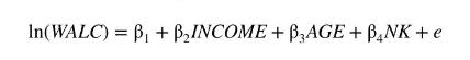
Does having more children drive parents to drink more alcohol? We have data on the following variables: \(W A L C=\) budget share (percent of income spent) for alcohol expenditure; INCOME = total net household income (10,000 UK pounds); \(A G E=\) age of household head \(/ 10 ; N K=\) number of children (1 or 2 ). We are interested in the equation

a. The data we have is based on a survey. If we hope to establish a causal relationship between \(N K\) and the budget share spent on alcohol, what assumptions are sufficient to prove that the least squares estimator is BLUE?

b. Using 1278 observations on households with a positive budget share for alcohol, the OLS estimated equation, with conventional standard errors, is

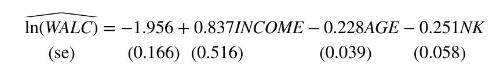
Test the null hypothesis that an increase in the number of children from one to two has no effect on the budget share of alcohol versus the alternative that an increase in the number of children increases the budget share of alcohol. Use the \(5 \%\) level of significance.

c. We suspect that the regression error variance might be larger for households with two children rather than one. We estimate the budget share equation by least squares separately for households with one and two children. For the 489 households with one child, the sum of squared residuals is 465.83. For the 789 households with two children, the sum of squared residuals is 832.77. Test the null hypothesis that there is no difference between the regression error variances for these two groups, against the alternative that there is a difference. Use the Goldfeld-Quandt test at the 5\% level of significance. Repeat the test using the alternative that the regression error variance for the subsample of households with two children is greater than the regression error variance for the subsample of households with one child. What do you conclude?

d. We save the least squares residuals from the estimation in part (b), calling them EHAT. We then obtain the second-stage regression results \(E H A T^{2}=0.012+0.279 A G E+0.025 N K\) with an \(R^{2}=0.0208\). Is there evidence of heteroskedasticity? Set up the appropriate hypothesis and carry out the test at the \(1 \%\) level of significance. What do you conclude?

e. We then carry out the regression \(\widehat{\ln \left(E H A T^{2}\right)}=-2.088+0.291 A G E-0.048 N K\). Holding \(N K\) constant, calculate the estimated variance ratio \(\widehat{\operatorname{var}}\left(e_{i} \mid A G E=40\right) / \widehat{\operatorname{var}}\left(e_{i} \mid A G E=30\right)\). What is the estimated ratio \(\widehat{\operatorname{var}}\left(e_{i} \mid A G E=60\right) / \widehat{\operatorname{var}}\left(e_{i} \mid A G E=30\right)\) ? Holding \(A G E\) constant, calculate the estimated variance ratio \(\widehat{\operatorname{var}}\left(e_{i} \mid N K=2\right) / \widehat{\operatorname{var}}\left(e_{i} \mid N K=1\right)\).

f. Based on the results we have obtained so far, can we claim that the least squares estimator used in (b) is BLUE?

g. What model would we estimate by OLS to implement feasible generalized least squares estimation?

Transcribed Image Text:

In(WALC) = B + BINCOME + BAGE + BANK + e