McCarthy and Ryan (1976) considered a model of television ownership in the United Kingdom and Ireland using data from 1955 to 1973 . Use the data file \(t v d a t a\) for this exercise.

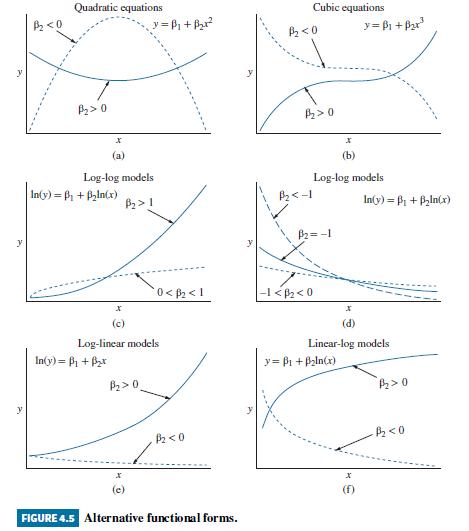
a. For the United Kingdom, plot the rate of television ownership (RATE_UK) against per capita consumer expenditures (SPEND_UK). Which models in Figure 4.5 are candidates to fit the data?

b. Estimate the linear-log model \(R A T E_{-} U K=\beta_{1}+\beta_{2} \ln \left(S P E N D_{-} U K\right)+e\). Obtain the fitted values and plot them against SPEND_UK. How well does this model fit the data?

c. What is the interpretation of the intercept in the linear-log model? Specifically, for the model in (b), for what value of \(S P E N D_{-} U K\) is the expected value \(E\left(R A T E \_U K \mid S P E N D \_U K\right)=\beta_{1}\) ?

d. Estimate the linear-log model RATE_UK \(=\beta_{1}+\beta_{2} \ln \left(S P E N D_{-} U K-280\right)+e\). Obtain the fitted values and plot them against SPEND_UK. How well does this model fit the data? How has the adjustment ( -280 ) changed the fitted relationship? [Note: You might well wonder how the value 280 was determined. It was estimated using a procedure called nonlinear least squares. You will be introduced to this technique later in this book.]

e. A competing model is the log-reciprocal model, described in Exercise 4.15. Estimate the log-reciprocal model \(\ln \left(R A T E \_U K\right)=\alpha_{1}+\alpha_{2}\left(1 / S P E N D \_U K\right)+e\). Obtain the fitted values and plot them against \(S P E N D \_U K\). How well does this model fit the data?

f. Explain the failure of the model in (e) by referring to Exercise 4.15(c).

g. Estimate the log-reciprocal model \(\ln \left(R A T E \_U K\right)=\alpha_{1}+\alpha_{2}\left(1 /\left[S P E N D_{-} U K-280\right]\right)+e\). Obtain the fitted values and plot them against SPEND_UK. How well does this model fit the data? How has this modification corrected the problem identified in part (f)?
h. Repeat the above exercises for Ireland, with correcting factor 240 instead of 280.

Data From Above Exercise:-

In Section 4.6, we considered the demand for edible chicken, which the U.S. Department of Agriculture calls "broilers." The data for this exercise are in the file newbroiler.

a. Using the 52 annual observations, 1950-2001, estimate the reciprocal model \(Q=\alpha_{1}+\) \(\alpha_{2}(1 / P)+e\). Plot the fitted value of \(Q=\) per capita consumption of chicken, in pounds, versus \(P=\) real price of chicken. How well does the estimated relation fit the data?

b. Using the estimated relation in part (a), compute the elasticity of per capita consumption with respect to real price when the real price is its median, \(\$ 1.31\), and quantity is taken to be the corresponding value on the fitted curve.

Compare this estimated elasticity to the estimate found in Section 4.6 where the \(\log\)-log functional form was used.

c. Estimate the poultry consumption using the linear-log functional form \(Q=\gamma_{1}+\gamma_{2} \ln (P)+e\). Plot the fitted values of \(Q=\) per capita consumption of chicken, in pounds, versus \(P=\) real price of chicken. How well does the estimated relation fit the data?

d. Using the estimated relation in part (c), compute the elasticity of per capita consumption with respect to real price when the real price is its median, \\($1.31\). Compare this estimated elasticity to the estimate from the log-log model and from the reciprocal model in part (b).

e. Estimate the poultry consumption using a log-linear model \(\ln (Q)=\phi_{1}+\phi_{2} P+e\). Plot the fitted values of \(Q=\) per capita consumption of chicken, in pounds, versus \(P=\) real price of chicken. How well does the estimated relation fit the data?

f. Using the estimated relation in part (e), compute the elasticity of per capita consumption with respect to real price when the real price is its median, \\($1.31\). Compare this estimated elasticity to the estimate from the previous models.

g. Evaluate the suitability of the alternative models for fitting the poultry consumption data, including the log-log model. Which of them would you select as best, and why?

Data From Exercise 4.15:-

Consider a log-reciprocal model that relates the logarithm of the dependent variable to the reciprocal of the explanatory variable, \(\ln (y)=\beta_{1}+\beta_{2}(1 / x)\).

a. For what values of \(y\) is this model defined? Are there any values of \(x\) that cause problems?

b. Write the model in exponential form as \(y=\exp \left[\beta_{1}+\beta_{2}(1 / x)\right]\). Show that the slope of this relationship is \(d y / d x=\exp \left[\beta_{1}+\left(\beta_{2} / x\right)\right] \times\left(-\beta_{2} / x^{2}\right)\). What sign must \(\beta_{2}\) have for \(y\) and \(x\) to have a positive relationship, assuming that \(x>0\) ?

c. Suppose that \(x>0\) but it converges toward zero from above. What value does \(y\) converge to? What does \(y\) converge to as \(x\) approaches infinity?

d. Suppose \(\beta_{1}=0\) and \(\beta_{2}=-4\). Evaluate the slope at the \(x\)-values \(0.5,1.0,1.5,2.0,2.5,3.0,3.5,4.0\). As \(x\) increases, is the slope of the relationship increasing or decreasing, or both?

e. Show that the second derivative of the function is

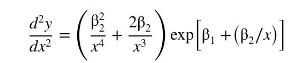
Assuming \(\beta_{2}0\), set the equation to zero, and show that the \(x\)-value that makes the second derivative zero is \(-\beta_{2} / 2\). Does this result agree with your calculations in part (d)?

Data From Figure 4.5:-

Transcribed Image Text:

dy B2B dx 202 exp[P + (P/x)]