Reconsider Example 6.19 where we used nonlinear least squares to estimate the model \(y_{i}=\beta x_{i 1}+\) \(\beta^{2} x_{i 2}+e_{i}\) by minimizing the sum of squares function \(S(\beta)=\sum_{i=1}^{N}\left(y_{i}-\beta x_{i 1}-\beta^{2} x_{i 2}\right)^{2}\).

a. Show that \(\frac{d S}{d \beta}=-2 \sum_{i=1}^{N} x_{i 1} y_{i}+2 \beta\left(\sum_{i=1}^{N} x_{i 1}^{2}-2 \sum_{i=1}^{N} x_{i 2} y_{i}\right)+6 \beta^{2} \sum_{i=1}^{N} x_{i 1} x_{i 2}+4 \beta^{3} \sum_{i=1}^{N} x_{i 2}^{2}\)

b. Show that \(\frac{d^{2} S}{d \beta^{2}}=2\left(\sum_{i=1}^{N} x_{i 1}^{2}-2 \sum_{i=1}^{N} x_{i 2} y_{i}\right)+12 \beta \sum_{i=1}^{N} x_{i 1} x_{i 2}+12 \beta^{2} \sum_{i=1}^{N} x_{i 2}^{2}\)

c. Given that \(\sum_{i=1}^{N} x_{i 1}^{2}=10.422155, \quad \sum_{i=1}^{N} x_{i 2}^{2}=3.586929, \quad \sum_{i=1}^{N} x_{i 1} x_{i 2}=4.414097, \quad \sum_{i=1}^{N} x_{i 1} y_{i}=\) 16.528022, and \(\sum_{i=1}^{N} x_{i 2} y_{i}=10.619469\), evaluate \(d S / d \beta\) at both the global minimum \(\beta=1.161207\) and at the local minimum \(\beta=-2.029494\). What have you discovered?

d. Evaluate \(d^{2} S / d \beta^{2}\) at both \(\beta=1.161207\) and \(\beta=-2.029494\).

e. At the global minimum, we find \(\hat{\sigma}_{G}=0.926452\) whereas, if we incorrectly use the local minimum, we find \(\hat{\sigma}_{L}=1.755044\). Evaluate

at both the global and local minimizing values for \(\beta\) and \(\hat{\sigma}\). What is the relevance of these values of \(q\) ? Go back and check Example 6.19 to see what you have discovered.

Data From Example 6.19:-

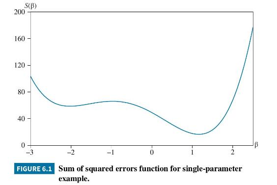
To illustrate estimation of (6.50), we use data stored in the file nlls. The sum of squared error function is graphed in Figure 6.1. Because we only have one parameter, we have a two-dimensional curve, not a "bowl." It is clear from the curve that the minimizing value for \(\beta\) lies between 1.0 and 1.5. From your favorite software, the nonlinear least squares estimate turns out to be \(b=1.1612\). The standard error depends on the degree of curvature of the sum of squares function at its minimum. A sharp minimum with a high degree of curvature leads to a relatively small standard error, while a flat minimum with a low degree of curvature leads to a relatively high standard error. There are different ways of measuring the curvature that can lead to different standard errors. In this example, the "outer-product of gradient" method yields a standard error of \(\operatorname{se}(b)=0.1307\), while the standard error from the "observed-Hessian" method is \(\operatorname{se}(b)=0.1324 .{ }^{12}\) Differences such as this one disappear as the sample size gets larger.
Two words of warning must be considered when estimating a nonlinear-in-the-parameters model. The first is to check that the estimation process has converged to a global minimum. The estimation process is an iterative one where a series of different parameter values are checked until the process converges at the minimum. If your software tells you the process has failed to converge, the output provided, if any, does not provide the nonlinear least squares estimates. This might happen if a maximum number of iterations has been reached or there has been a numerical problem that has caused the iterations to stop. A second problem that can occur is that the iterative process may stop at a "local" minimum rather than the "global" minimum. In the example in Figure 6.1, there is a local minimum at \(\beta=-2.0295\). Your software will have an option of giving starting values to the iterative process. If you give it a starting value of -2 , it is highly likely you will end up with the estimate \(b=-2.0295\). This value is not the nonlinear least squares estimate, however. The nonlinear least squares estimate is at the global minimum which is the smallest of the minima if more than one exists. How do you guard against ending up at a local minimum? It is wise to try different starting values to ensure you end up at the same place each time. Notice that the curvature at the local minimum in Figure 6.1 is much less than at the global minimum. This should be reflected in a larger "standard error" at the local minimum. Such is indeed the case. We find the outer-product-gradient method yields \(\operatorname{se}(b)=0.3024\), and from the observed-Hessian method we obtain \(\operatorname{se}(b)=0.3577\).

Data From Equation 6.50:-

Transcribed Image Text:

9= 2 dS/d$?