For the Hausman test given in Section 8.4.1 let (mathrm{V}_{11}=mathrm{V}[widehat{theta}], mathrm{V}_{22}=mathrm{V}[tilde{theta}]), and (mathrm{V}_{12}=operatorname{Cov}[widehat{boldsymbol{theta}}, tilde{boldsymbol{theta}}]). (a) Show that the estimator (bar{theta}=widehat{boldsymbol{theta}}+left[mathrm{V}_{11}+mathrm{V}_{22}-2 mathrm{~V}_{12} ight]^{-1}(tilde{boldsymbol{theta}}, widehat{boldsymbol{theta}})) has asymptotic

For the Hausman test given in Section 8.4.1 let \(\mathrm{V}_{11}=\mathrm{V}[\widehat{\theta}], \mathrm{V}_{22}=\mathrm{V}[\tilde{\theta}]\), and \(\mathrm{V}_{12}=\operatorname{Cov}[\widehat{\boldsymbol{\theta}}, \tilde{\boldsymbol{\theta}}]\).

(a) Show that the estimator \(\bar{\theta}=\widehat{\boldsymbol{\theta}}+\left[\mathrm{V}_{11}+\mathrm{V}_{22}-2 \mathrm{~V}_{12}\right]^{-1}(\tilde{\boldsymbol{\theta}}, \widehat{\boldsymbol{\theta}})\) has asymptotic variance matrix \(V[\bar{\theta}]=\mathrm{V}_{11}-\left[\mathrm{V}_{11}-\mathrm{V}_{12}\right]\left[\mathrm{V}_{11}+\mathrm{V}_{22}-2 \mathrm{~V}_{12}\right]^{-1}\left[\mathrm{~V}_{11}-\mathrm{V}_{12}\right]\).

(b) Hence show that \(V[\bar{\theta}]\) is less than \(V[\widehat{\theta}]\) in the matrix sense unless \(\operatorname{Cov}[\hat{\theta}, \widetilde{\theta}]=\) \(\mathrm{V}[\widehat{\theta}]\).

(c) Now suppose that \(\widehat{\theta}\) is fully efficient. Can \(V[\bar{\theta}]\) be less than \(\mathrm{V}[\widehat{\theta}]\) ? What do you conclude?

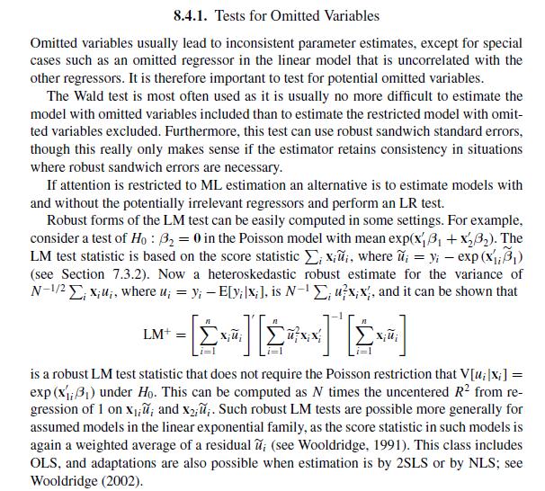
8.4.1. Tests for Omitted Variables Omitted variables usually lead to inconsistent parameter estimates, except for special cases such as an omitted regressor in the linear model that is uncorrelated with the other regressors. It is therefore important to test for potential omitted variables. The Wald test is most often used as it is usually no more difficult to estimate the model with omitted variables included than to estimate the restricted model with omit- ted variables excluded. Furthermore, this test can use robust sandwich standard errors, though this really only makes sense if the estimator retains consistency in situations where robust sandwich errors are necessary. If attention is restricted to ML estimation an alternative is to estimate models with and without the potentially irrelevant regressors and perform an LR test. Robust forms of the LM test can be easily computed in some settings. For example, consider a test of Ho: 32 = 0 in the Poisson model with mean exp(x1+x232). The LM test statistic is based on the score statistic xiui, where ; = y; - exp (x1, B) (see Section 7.3.2). Now a heteroskedastic robust estimate for the variance of N-1/2 2; x;u;, where u; = y; -Elyx;], is N, ux,x, and it can be shown that 11 LM+= is a robust LM test statistic that does not require the Poisson restriction that V[u; [xi] = exp (x1,) under Ho. This can be computed as N times the uncentered R from re- gression of 1 on x;u; and X2;u;. Such robust LM tests are possible more generally for assumed models in the linear exponential family, as the score statistic in such models is again a weighted average of a residual u; (see Wooldridge, 1991). This class includes OLS, and adaptations are also possible when estimation is by 2SLS or by NLS; see Wooldridge (2002).