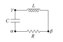
Consider an L-C-R circuit as shown in Fig. 6.15. This circuit is governed by the differential equation (6.72), where F´ is the fluctuating voltage produced by the resistor’s microscopic degrees of freedom (so we shall rename it V´), and F ≡ V vanishes, since there is no driving voltage in the circuit. Assume that the resistor has temperature T >> ℏω_o/k, where ω_o = (LC)^−1/2 is the circuit’s resonant angular frequency, ω_o = 2πf_o, and also assume that the circuit has a large quality factor (weak damping) so R ≪ 1/(ω_oC) ≈ ω_oL.

(a) Initially consider the resistor R decoupled from the rest of the circuit, so current cannot flow across it. What is the spectral density V_αβ of the voltage across this resistor?

(b) Now place the resistor into the circuit as shown in Fig. 6.15. The fluctuating voltage V´ will produce a fluctuating current I = q̇ in the circuit (where q is the charge on the capacitor).What is the spectral density of I? And what, now, is the spectral density V_αβ across the resistor?

(c) What is the spectral density of the voltage V_αγ between points α and γ? and of V_βγ ?

(d) The voltage V_αβ is averaged from time t = t₀ to t = t₀ + τ (with τ >> 1/f_o), giving some average value U₀. The average is measured once again from t₁ to t₁ + τ , giving U₁. A long sequence of such measurements gives an ensemble of numbers {U₀, U₁, . . . , U_n}. What are the mean U̅ and rms deviation △U ≡ ((U − U̅)²)1/2 of this ensemble?

Equation 6.72

Fig 6.15

Transcribed Image Text:

Lä+C¹q = Fbath (t) = −Rġ + F', (6.72)