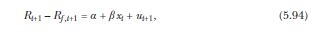
In this exercise we study empirically whether the out-of-sample stock market return predictability of well-known valuation ratios can be improved by imposing simple theoretical restrictions on the predictive regressions. The data for this question can be found in an Excel spreadsheet on the textbook website \({ }^{10}\) together with an accompanying explanatory document offering more details on the suggested implementation of the predictive regressions. Consider the regression

where \(R_{t+1}\) denotes the one-quarter-ahead return to the S\&P 500 index and \(x_{t}\) is a predictor variable. Motivated by the claim of Welch and Goyal (2008) that the historical average excess stock return forecasts future excess stock returns out of sample better than regressions of excess returns on predictor variables, we evaluate the out-of-sample performance of forecasts based on predictor variable \(x_{t}\) using the out-of-sample \(R^{2}\) statistic computed as

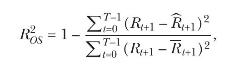
where \(\widehat{R}_{t+1}\) is the fitted value from regression (5.94) estimated from the start date \(-T_{I E}\) of the initial estimation sample through date \(t\) and \(\bar{R}_{t+1}\) is the historical arithmetic average return estimated from \(-T_{I E}\) through \(t\). Here \(T_{I E}\) is the length of the initial estimation period, and \(T\) is the length of the out-of-sample forecast evaluation period. A positive value for \(R_{O S}^{2}\) means that the predictive regression has lower average mean-squared prediction error than the historical average return.

(a) Calculate the in-sample \(R^{2}\) statistics for the dividend yield, \(x_{t}=D_{t} / P_{t}\), and the smoothed earnings yield, \(x_{t}=X_{t} / P_{t}\), when regression (5.94) is estimated by standard ordinary least squares (OLS) over the full sample from 1872 to 2016.

Equation 5.94

(b) Calculate the out-of-sample \(R^{2}\) statistics for the two valuation ratios when regression (5.94) is estimated by standard OLS, with 1872-1926 as the initial estimation period and 1927-2016 as the out-of-sample forecast evaluation period.
Compare the values you obtained for the in-sample and out-of-sample \(R^{2}\) statistics. Are your results consistent with Welch and Goyal's (2008) claim?

(c) Repeat the calculations of the previous part for the out-of-sample \(R^{2}\) statistics but now impose the (rather weak) theoretical restrictions that the slope \(\beta\) in the predictive regression and the forecast for the excess return are both nonnegative. That is, calculate the return forecast as

where \(\widehat{\alpha}_{t+1}\) and \(\widehat{\beta}_{t+1}\) denote the intercept and slope estimates from the standard OLS regression and \(\bar{x}_{t+1}\) is the historical arithmetic average value of \(x\), all estimated through period \(t\).
Is there a significant improvement in the out-of-sample explanatory power of the two valuation ratios?
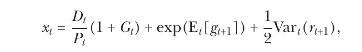
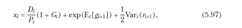
In the remaining parts of the exercise, we examine whether the forecasting performance of the dividend yield improves once we impose the theoretical restrictions of the drifting steady-state valuation model of section 5.5.2. Following equation (5.87), we use a version of the dividend yield adjusted for dividend growth and the real rate as our predictor variable:

Equation 5.87

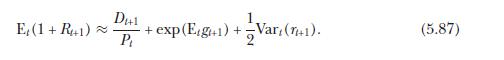
where \(\mathrm{E}_{t}\left[g_{t+1}ight]\) and \(\operatorname{Var}_{t}\left(r_{t+1}ight)\) denote market participants' conditional expectation of future log dividend growth and the conditional variance of log returns.

(d) Construct an estimate of (5.97) using the historical sample mean of dividend growth and the historical sample variance of log stock returns up to date \(t\). Even though the model assumes that market participants know the value of \(D_{t+1}\) at date \(t\), to avoid any look-ahead bias construct a real-time estimate of \(x_{t}\) assuming that \(D_{t+1}\) is not in the econometrician's information set at date \(t\).
Discuss alternative procedures that you could use to construct real-time estimates of \(\mathrm{E}_{t}\left[g_{t+1}ight]\) and \(\operatorname{Var}_{t}\left(r_{t+1}ight)\).

(e) Repeat the calculations of parts

(b) and

(c) for \(x_{t}\) given by (5.97). Compare the forecasting performance of this adjusted version of the dividend yield with that of the (unadjusted) dividend yield.

(f) Finally, fully impose the theoretical restriction of equation (5.97) by calculating the predicted return as \({ }^{11}\)

Equation 5.97

where \(x_{t}\) is given by (5.97). What is the out-of-sample \(R^{2}\) statistic now? Discuss your conclusions from this exercise.

Data from section 5.5.2

Transcribed Image Text:

R-1-R+a+Bx + U+13