We consider the following portfolio optimization problem:

where C is the empirical covariance matrix, A > 0 is a risk parameter and r̂ is the time-average return for each asset for the given period. Here, the constraint set X is determined by the following conditions.

• No shorting is allowed.
• There is a budget constraint X_i + • • • + x_n = 1.

In the above, the function T represents transaction costs and market impact, c ≥ 0 is a parameter that controls the size of these costs, while x° ∈ Rⁿ is the vector of initial positions. The function T has the form 

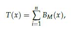
where the function B_M is piece-wise linear for small x, and quadratic for large x; that way we seek to capture the fact that transaction costs are dominant for smaller trades, while market impact kicks in for larger ones. Precisely, we define B_M to be the so-called "reverse Huber" function with cut-off parameter M: for a scalar z, the function value is 

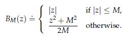
The scalar M > 0 describes where the transition from a linearly shaped to a quadratically shaped penalty takes place.
1. Show that B_M can be expressed as the solution to an optimization problem:

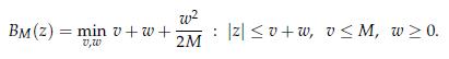
Explain why the above representation proves that B_M is convex.

2. Show that, for given x ∈ Rⁿ:

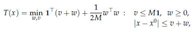
where, in the above, ν,ω are now n-dimensional vector variables, 1 is the vector of ones, and the inequalities are component-wise. 

3. Formulate the optimization problem (14.40) in convex format. Does the problem fall into one of the categories (LP, QP, SOCP, etc) seen in Chapter 8? 

max Tx - AxTCx-c-T(x-x): x 0, x= x,