

Question: 2. Test whether there is an association between a person's educational attainment and how much television they watch. Use the GSS08 data set to
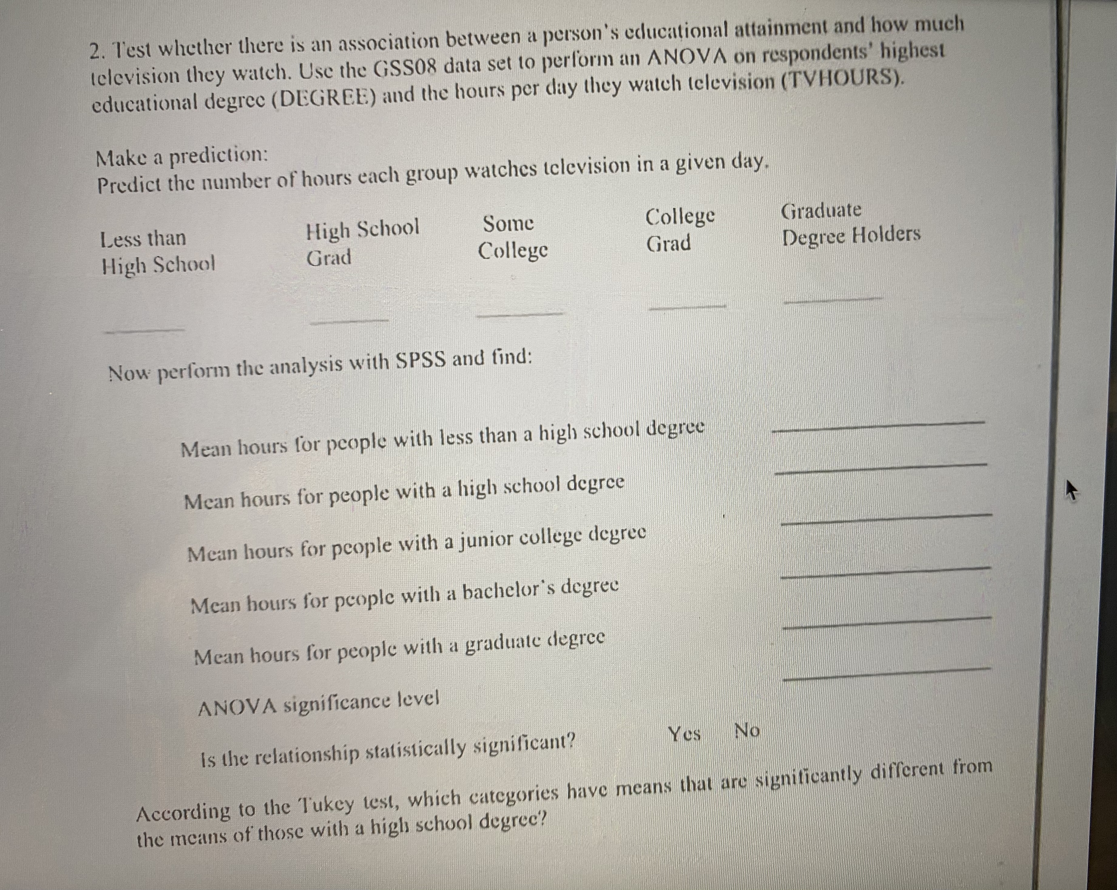
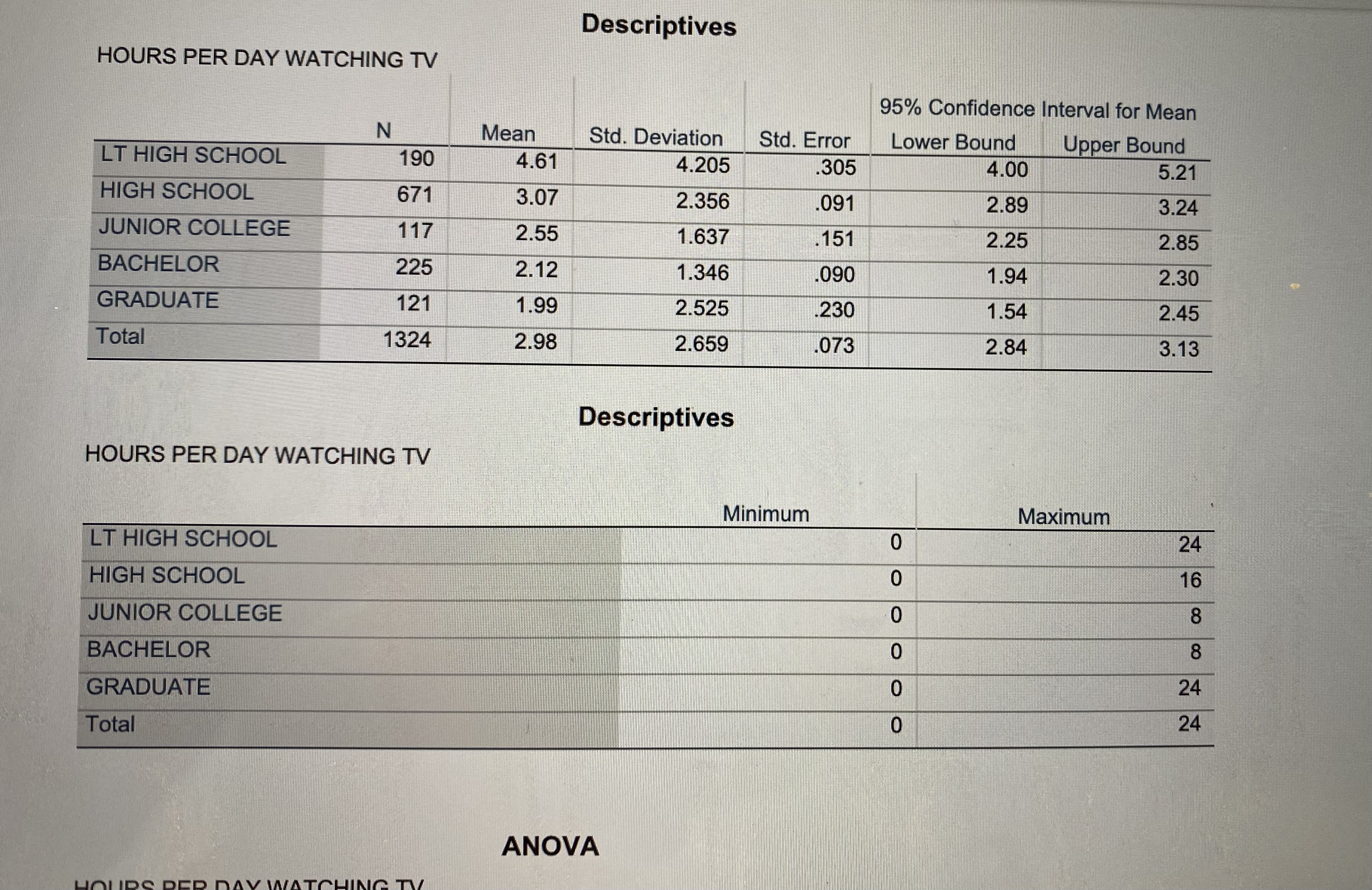
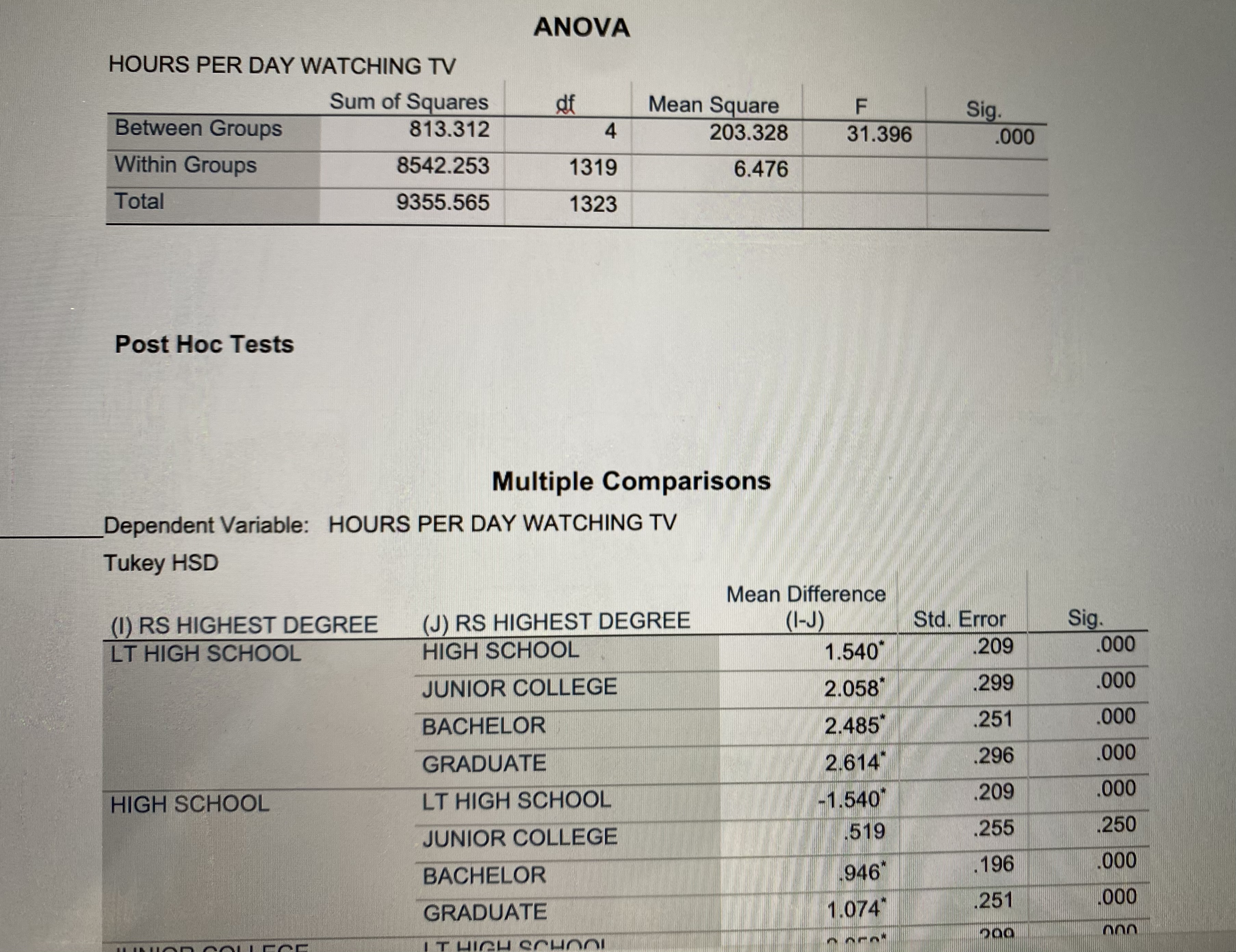
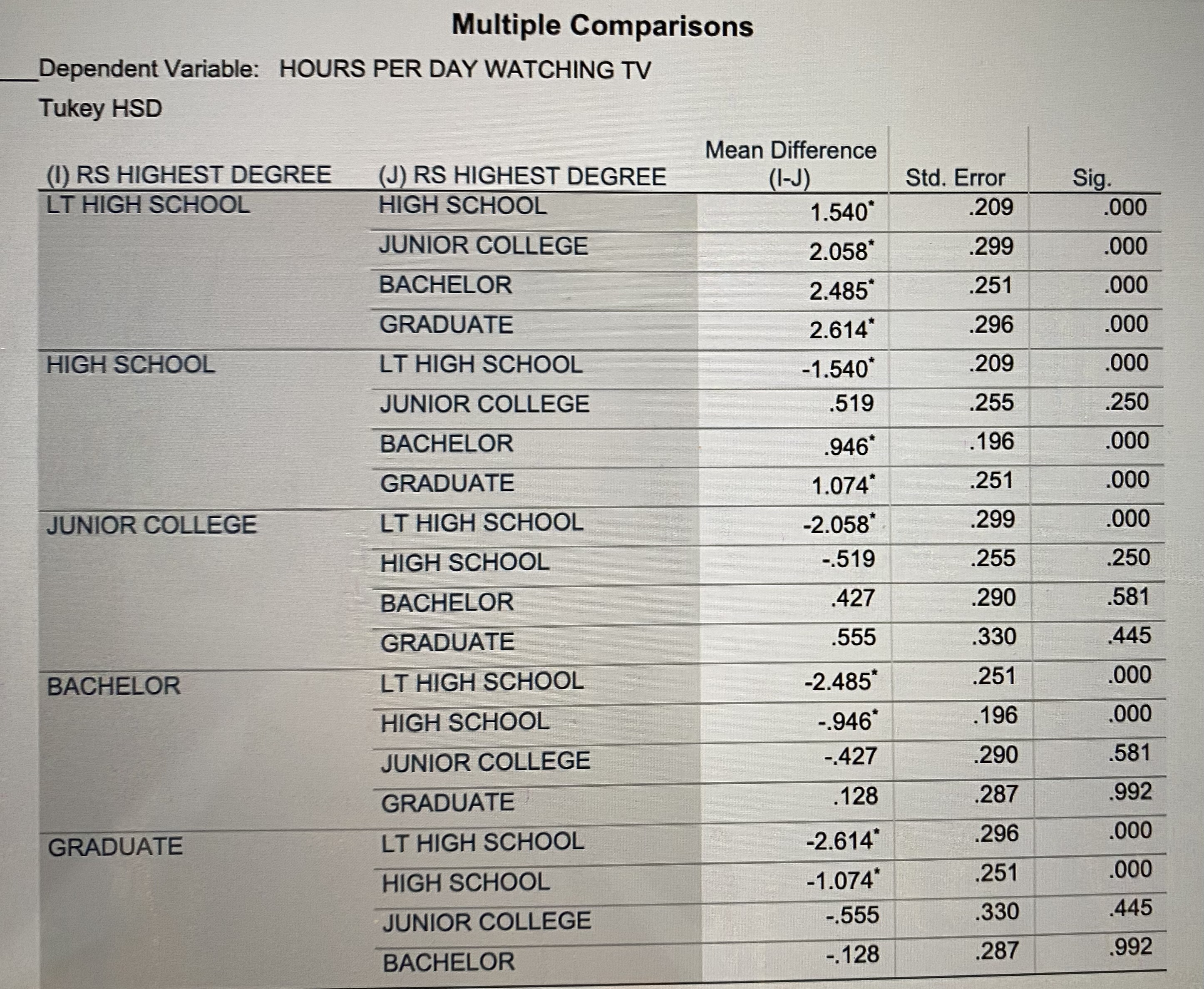
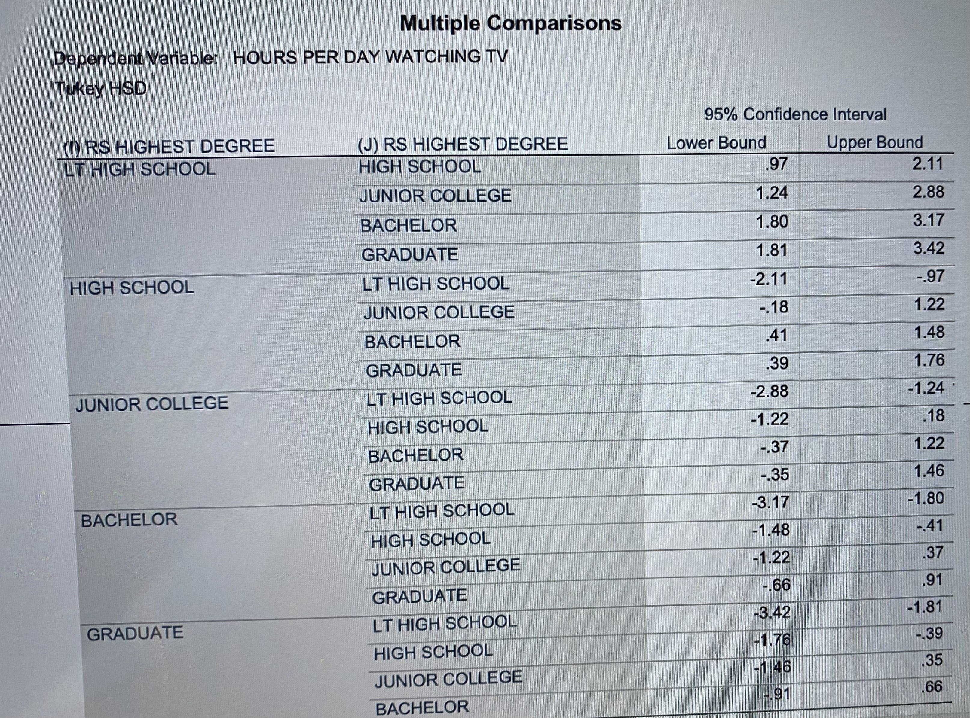
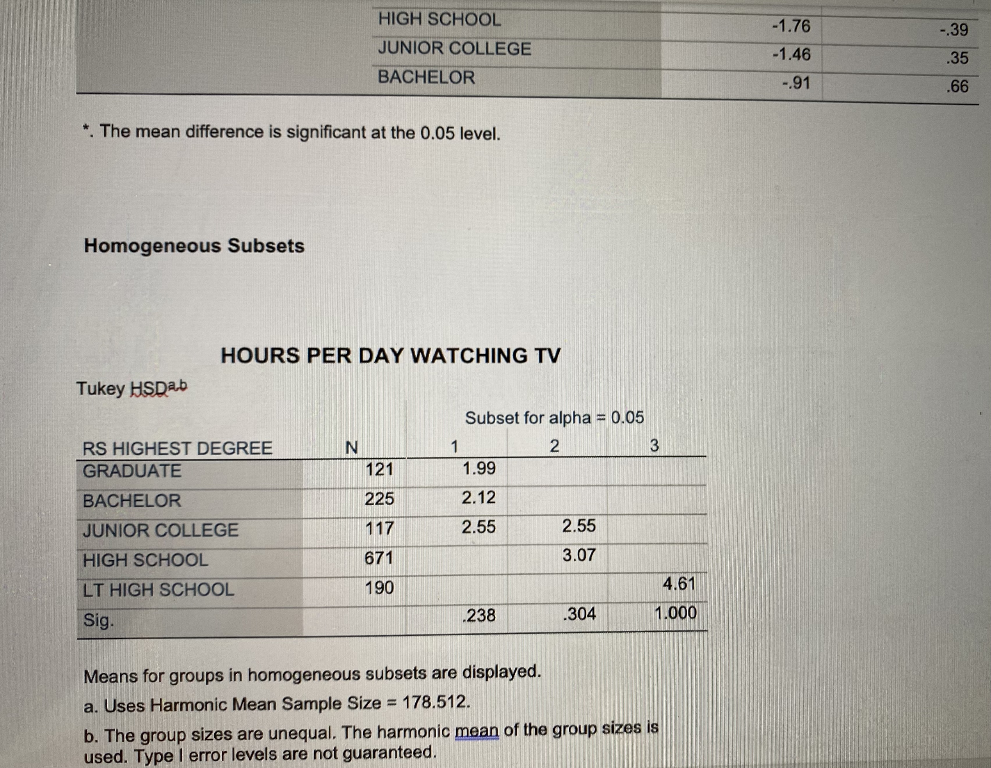
2. Test whether there is an association between a person's educational attainment and how much television they watch. Use the GSS08 data set to perform an ANOVA on respondents' highest educational degree (DEGREE) and the hours per day they watch television (TVHOURS). Make a prediction: Predict the number of hours each group watches television in a given day. Less than High School High School Grad Some College College Grad Now perform the analysis with SPSS and find: Mean hours for people with less than a high school degree Mean hours for people with a high school degree Mean hours for people with a junior college degree Mean hours for people with a bachelor's degree Mean hours for people with a graduate degree ANOVA significance level Is the relationship statistically significant? Yes No Graduate Degree Holders According to the Tukey test, which categories have means that are significantly different from the means of those with a high school degree? HOURS PER DAY WATCHING TV Descriptives 95% Confidence Interval for Mean N Mean Std. Deviation Std. Error Lower Bound Upper Bound LT HIGH SCHOOL 190 4.61 4.205 .305 4.00 5.21 HIGH SCHOOL 671 3.07 2.356 .091 2.89 3.24 JUNIOR COLLEGE 117 2.55 1.637 .151 2.25 2.85 BACHELOR 225 2.12 1.346 .090 1.94 2.30 GRADUATE 121 1.99 2.525 .230 1.54 2.45 Total 1324 2.98 2.659 .073 2.84 3.13 HOURS PER DAY WATCHING TV LT HIGH SCHOOL HIGH SCHOOL JUNIOR COLLEGE BACHELOR GRADUATE Total HOURS PER DAY WATCHING TV Descriptives ANOVA Minimum 00000 0 Maximum 24 16 8 8 24 24 HOURS PER DAY WATCHING TV ANOVA Sum of Squares df Mean Square F Sig. Between Groups 813.312 4 203.328 31.396 .000 Within Groups 8542.253 1319 6.476 Total 9355.565 1323 Post Hoc Tests Multiple Comparisons Dependent Variable: HOURS PER DAY WATCHING TV Tukey HSD (I) RS HIGHEST DEGREE LT HIGH SCHOOL (J) RS HIGHEST DEGREE HIGH SCHOOL Mean Difference (1-J) Std. Error Sig. 1.540 209 .000 JUNIOR COLLEGE 2.058" .299 .000 BACHELOR 2.485 .251 .000 GRADUATE 2.614" .296 .000 HIGH SCHOOL LT HIGH SCHOOL -1.540 .209 .000 JUNIOR COLLEGE 519 .255 .250 BACHELOR 946 196 .000 GRADUATE 1.074 251 .000 200 000 IT HIGH SCHOOL Multiple Comparisons Dependent Variable: HOURS PER DAY WATCHING TV Tukey HSD Mean Difference (I) RS HIGHEST DEGREE LT HIGH SCHOOL (J) RS HIGHEST DEGREE (I-J) Std. Error Sig. HIGH SCHOOL 1.540* .209 .000 JUNIOR COLLEGE 2.058* .299 .000 BACHELOR 2.485* .251 .000 GRADUATE 2.614* .296 .000 HIGH SCHOOL LT HIGH SCHOOL -1.540* .209 .000 JUNIOR COLLEGE .519 .255 .250 BACHELOR .946* .196 .000 GRADUATE 1.074* .251 .000 JUNIOR COLLEGE LT HIGH SCHOOL -2.058* .299 .000 HIGH SCHOOL -.519 .255 .250 BACHELOR .427 .290 .581 GRADUATE .555 .330 .445 BACHELOR LT HIGH SCHOOL -2.485* .251 .000 HIGH SCHOOL -.946* .196 .000 JUNIOR COLLEGE -.427 .290 .581 GRADUATE .128 .287 .992 GRADUATE LT HIGH SCHOOL -2.614* .296 .000 HIGH SCHOOL -1.074* .251 .000 JUNIOR COLLEGE -.555 .330 .445 BACHELOR -.128 .287 .992 Multiple Comparisons Dependent Variable: HOURS PER DAY WATCHING TV Tukey HSD 95% Confidence Interval (1) RS HIGHEST DEGREE LT HIGH SCHOOL (J) RS HIGHEST DEGREE HIGH SCHOOL Lower Bound Upper Bound .97 2.11 JUNIOR COLLEGE BACHELOR 1.24 2.88 1.80 3.17 GRADUATE 1.81 3.42 HIGH SCHOOL LT HIGH SCHOOL -2.11 -.97 JUNIOR COLLEGE -.18 1.22 BACHELOR .41 1.48 GRADUATE .39 1.76 JUNIOR COLLEGE LT HIGH SCHOOL -2.88 -1.24 1 HIGH SCHOOL -1.22 .18 BACHELOR -.37 1.22 GRADUATE -.35 1.46 BACHELOR LT HIGH SCHOOL -3.17 -1.80 HIGH SCHOOL -1.48 -.41 JUNIOR COLLEGE -1.22 .37 GRADUATE -.66 .91 GRADUATE LT HIGH SCHOOL -3.42 -1.81 HIGH SCHOOL -1.76 -.39 JUNIOR COLLEGE -1.46 35 -.91 66 BACHELOR HIGH SCHOOL -1.76 -.39 JUNIOR COLLEGE BACHELOR -1.46 .35 -.91 .66 *. The mean difference is significant at the 0.05 level. Homogeneous Subsets HOURS PER DAY WATCHING TV Tukey HSDab Subset for alpha = 0.05 RS HIGHEST DEGREE N 1 2 3 GRADUATE 121 1.99 BACHELOR 225 2.12 JUNIOR COLLEGE 117 2.55 2.55 HIGH SCHOOL 671 3.07 LT HIGH SCHOOL 190 4.61 Sig. .238 .304 1.000 Means for groups in homogeneous subsets are displayed. a. Uses Harmonic Mean Sample Size = 178.512. b. The group sizes are unequal. The harmonic mean of the group sizes is used. Type I error levels are not guaranteed.
Step by Step Solution
There are 3 Steps involved in it

Get step-by-step solutions from verified subject matter experts