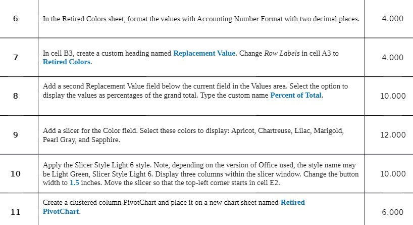
6 In the Retired Colors sheet, format the values with Accounting Number Format with two decimal places. 4.000 7 In cell B3, create a custom heading named Replacement Value. Change Row Labels in cell A3 to Retired Colors. 4.000 Add a second Replacement Value field below the current field in the Values area. Select the option to 8 display the values as percentages of the grand total. Type the custom name Percent of Total. 10.000 9 Add a slicer for the Color field. Select these colors to display: Apricot, Chartreuse, Lilac, Marigold, Pearl Gray, and Sapphire. 12.000 Apply the Slicer Style Light 6 style. Note, depending on the version of Office used, the style name may 10 be Light Green, Slicer Style Light 6. Display three columns within the slicer window. Change the button 10.000 width to 1.5 inches. Move the slicer so that the top-left corner starts in cell E2. Create a clustered column PivotChart and place it on a new chart sheet named Retired 11 PivotChart. 6.000