$($a$)$ Modify the function ex$\_$with$\_2$eqs to solve the IVP $(4)$ for $0t60$ using the MATLAB

routine ode$45.$ Call the new function LAB$04$ex$1.$

Let $t,Y($note the upper case $Y)$ be the output of ode$45$ and $y$ and $v$ the unknown functions.

Use the following commands to define the ODE:

function $dYdt=f(t,Y)$

$y=Y(1)$;$v=Y(2)$;

$dYdt=[v$;$-3**sin(t)-3**v-6**y]$;

Plot $y(t)$ and $v(t)$ in the same window $($do not use subplot$),$ and the phase plot showing $v$ vs

$y$ in a separate window.

Add a legend to the first plot. $($Note: to display $v(t)=y^{\text{'}}(t),$ use $\text{'}v(t)=y\text{'}\text{'}(t{)}^{\text{'}}\text{'}).$

Add a grid. Use the command ylim $([-2\mathrm{.}8,2\mathrm{.}8]$ to adjust the $y-$limits for both plots. Adjust

the $x-$limits in the phase plot so as to reproduce the pictures in Figure $7.$Figure $7$: Time series $y=y(t)$ and $v=v(t)=y^{\text{'}}(t)($left$),$ and phase plot $v=y^{\text{'}}$ vs$.y$ for $(4).$

$($b$)$ By reading the matrix $Y$ and the vector $t,$ find $($approximately$)$ the last three values of $t$ in

the interval $0t60$ at which $y$ reaches a local maximum. Note that, because the M$-$file

LAB$04$ex$1.$m is a function file, all the variables are local and thus not available in the Command

Window. To read the matrix $Y$ and the vector $t,$ you need to modify the M$-$file by adding the

line $t,Y($:$,1),Y($:$,2).$

Do not include the whole output in your lab write$-$up$.$ Include only the values necessary to

answer the question, i$.$e$.$ just the rows of $t,y,v$ with local $y-$maxima and the adjacent

rows. To quickly locate the desired rows, recall that the local maxima of a differentiable

function appear where its derivative changes sign from positive to negative. $($Note: Due to

numerical approximations and the fact that the numerical solution is not necessarily computed

at the exact $t-$values where the maxima occur, you should not expect $v(=y^{\text{'}})$ to be exactly $0$

at local maxima, but only close to $0).$

$($c$)$ What seems to be the long term behavior of $y?$

$($d$)$ Modify the initial conditions to $y(0)=-1\mathrm{.}2,v(0)=-1\mathrm{.}9$ and run the file LAB$04$ex$1.$m with

the modified initial conditions. Based on the new graphs, determine whether the long term

behavior of the solution changes. Explain. Include the pictures with the modified initial

conditions to support your answer.$t0=0$;$tf=20$;$y=[10$;$60]$;

$a=\mathrm{.}8$;$b=\mathrm{.}01$;$c=\mathrm{.}6$;$d=\mathrm{.}1$;

$[t,y]=$ode$45($@$f,[t,tf],y,[],a,b,c,d)$;

$u1=y($:$,1)$;$u2=y($:$,2)$;$,\%$ y in output has $2$ columns corresponding to $u1$ and $u2$

figure$(1)$;

subplot$(2,1,1)$; plot$($t$,$u$1,\text{'}$b$-+\text{'})$; ylabel$(\text{'}$u$1\text{'})$;

subplot$(2,1,2)$; plot$($t$,$u$2,\text{'}$ro$-\text{'})$; ylabel$(\text{'}$u$2\text{'})$;

figure$(2)$

plot$($u$1,$u$2)$; axis square; xlabel$(\text{'}$u$\_1\text{'})$; ylabel$(\text{'}$u$\_2\text{'})$; $\%$ plot the phase plot

$\%-$

function $dydt=f(t,y,a,b,c,d)$

$u1=y(1)$;$u2=y(2)$;

dydt $=[a**u1-b^{**}u{1}^{**}u2$;$-c^{**}u2+d**u1**u2]$;

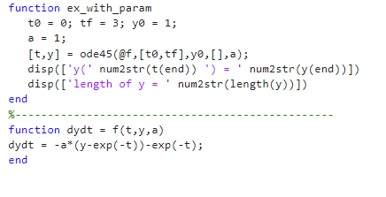
endfunction ex$\_$with$\_$param

$t=0$;$tf=3$;$y=1$;

$a=1$;

$[t,y]=$ode$45($@$f,[t,tf],y,[],a)$;

num end