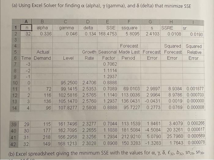
Question: (a) Using Excel Solver for finding a (alpha), y (gamma), and 8 (delta) that minimize SSE C gamma 0.046 E delta SSE 0.134 168.4753 ssquare
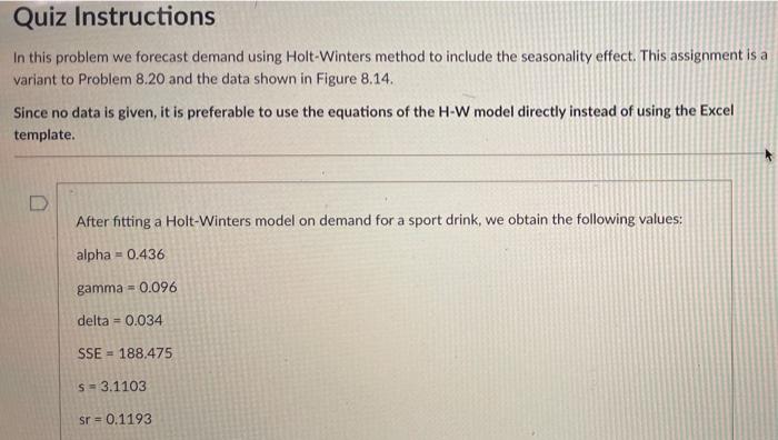
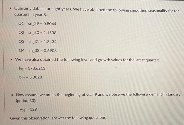
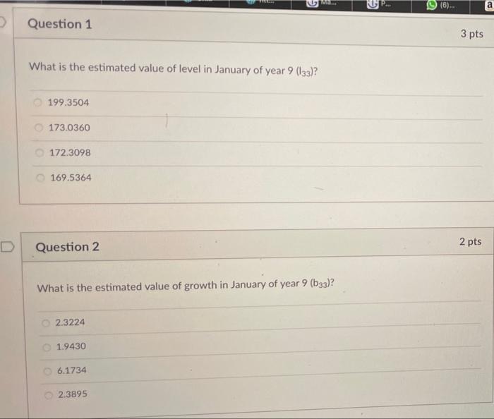
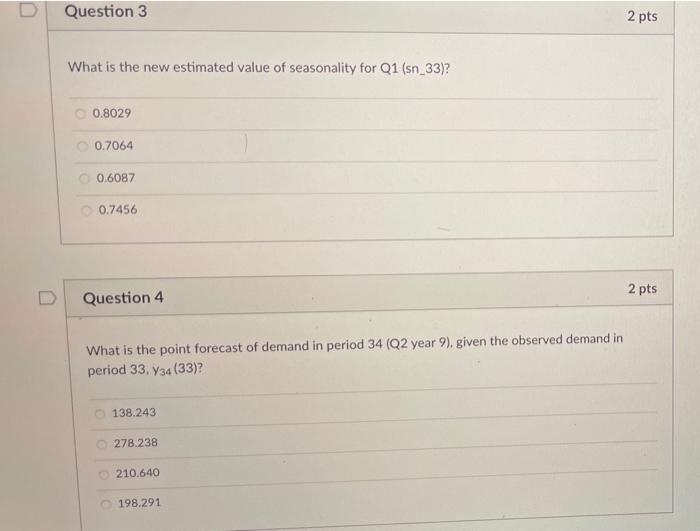
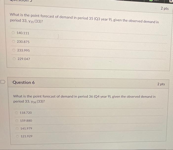
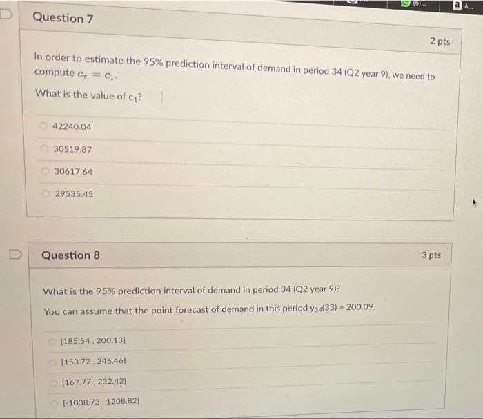
(a) Using Excel Solver for finding a (alpha), y (gamma), and 8 (delta) that minimize SSE C gamma 0.046 E delta SSE 0.134 168.4753 ssquare 5.8095 G H S SSRE sr 2.4103 0.0108 0.0193 0 h N A B 1 alpha 2 32 0.336 3 4 5 Actual 6 Time Demand 7 -3 8 -2 9 - 1 10 0 11 1 72 12 2 116 13 3 136 14 4 96 00 99 st Forecast Squared Squared Growth Seasonal Made Last Forecast Forecast Relative Level Rate Factor Period Error Error Error 0.7062 1.1114 1.2937 95.2500 2.4706 0.8886 99.1415 2.5353 0.7089 69.0103 2.9897 8.9384 0.001877 102 5816 2.5765 1.1140 113.0036 2.9964 8.9786 0.000703 105.1470 2.5760 1.2937 136.0431 -0.0431 0.0019 0.000000 107.8277 2.5808 0.8888 95.7227 0.2773 0.0769 0.000008 39 40 41 29 30 31 32 115 177 218 149 161.7496 2.3277 162.7095 2.2655 166 2958 2.3256 168.1213 2.3028 0.7044 113. 1539 1.8461 3.4079 0.000266 1.1038 181.5084 -4.5084 20.3261 0.000617 1.2934 212.9210 5.0790 25 7960 0.000569 0.8908 150.3283 -1.3283 1.7643 0.000078 42 (b) Excel spreadsheet giving the minimum SSE with the values for a 7, 8, 132, b32, sn 29, Sn 30 Quiz Instructions In this problem we forecast demand using Holt-Winters method to include the seasonality effect. This assignment is a variant to Problem 8.20 and the data shown in Figure 8.14. Since no data is given, it is preferable to use the equations of the H-W model directly instead of using the Excel template. After fitting a Holt-Winters model on demand for a sport drink, we obtain the following values: alpha=0.436 gamma = 0.096 delta = 0.034 SSE - 188.475 S = 3.1103 sr = 0.1193 Quarterly data is for eight years. We have obtained the following smoothed seasonality for the quarters in year 8. Q1 sn 29 = 0.8044 Q2 sn_30 = 1.1538 Q3 sn_31 = 1.3434 Q4sn_32 = 0.6908 We have also obtained the following level and growth values for the latest quarter: 132 = 173.6213 b32 = 3.0028 Now assume we are in the beginning of year 9 and we observe the following demand in January (period 33): Y33 = 129 Given this observation, answer the following questions. TV 19 (6)... a Question 1 3 pts What is the estimated value of level in January of year 9 (133)? 199.3504 173.0360 172.3098 169.5364 D 2 pts Question 2 What is the estimated value of growth in January of year 9 (633)? 2.3224 1.9430 6.1734 2.3895 D Question 3 2 pts What is the new estimated value of seasonality for Q1 (sn_33)? 0.8029 0.7064 0.6087 0.7456 2 pts Question 4 What is the point forecast of demand in period 34 (Q2 year 9), given the observed demand in period 33, 34 (33)? 138.243 278.238 210.640 198.291 2 pts What is the point forecast of demand in period 35 (Q3 year 9), given the observed demand in period 33, 735 (33)? 140.111 230.875 233.995 229.047 Question 6 2 pts What is the point forecast of demand in period 36 (Q4 year 9), given the observed demand in period 33.736 (33)? 118.720 159.880 141.979 121.929 TU.. a A. Question 7 2 pts In order to estimate the 95% prediction interval of demand in period 34 (Q2 year 9), we need to compute c = ci What is the value of ci? 42240.04 30519.87 30617.64 29535,45 Question 8 3 pts What is the 95% prediction interval of demand in period 34 (Q2 year 9)? You can assume that the point forecast of demand in this period Y34(33) - 200.09. (185.54.200.13] [153.72, 246.46] (167.77.232.42] [-1008.73.1208.82]