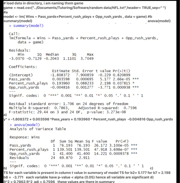
Question: ASAP please regression analysis Using the nfl.txt data set (a) Construct a normal probability plot of the residuals. Do there appear to be any issues

ASAP please

regression analysis

Using the nfl.txt data set

(a) Construct a normal probability plot of the residuals. Do there appear to be any issues with the normality assumption? Comment. (b) Construct and discuss a plot of the studentized residuals versus the fitted values. (c) Construct discuss plots of the residuals versus each of the predictors. Do these plots give any indications that the predictors are incorrectly specified? (d) Examine the studentized residuals for this model. What information is conveyed by them, and do they suggest any issues with these data?

nfl.text:

"Wins" "Rush.yards" "Pass.yards" "Punt.avg" "FG.." "Turnover.differential" "Penalty.yards" "Percent.rush.plays" "Opp.rush.yards" "Opp.Pass.yards" "Washington" 10 2113 1985 28.9 64.7 4 868 59.7 2205 1917 "Minnesota" 11 2003 2855 28.8 61.3 3 615 55 2096 1575 "New England" 11 2957 1737 40.1 60 14 914 65.6 1847 2175 "Oakland" 13 2285 2905 41.6 45.3 -4 957 61.4 1903 2476 "Pittsburgh" 10 2971 1666 39.2 53.8 15 836 66.1 1457 1866 "Baltimore" 11 2309 2927 39.7 74.1 8 786 61 1848 2339 "Los Angeles" 10 2528 2341 38.1 65.4 12 754 66.1 1564 2092 "Dallas" 11 2147 2737 37 78.3 -1 761 58 1821 1909 "Atlanta" 4 1689 1414 42.1 47.6 -3 714 57 2577 2001 "Buffalo" 2 2566 1838 42.3 54.2 -1 797 58.9 2476 2254 "Chicago" 7 2363 1480 37.3 48 19 984 67.5 1984 2217 "Cincinnati" 10 2109 2191 39.5 51.9 6 700 57.2 1917 1758 "Cleveland" 9 2295 2229 37.5 53.6 -5 1037 58.8 1761 2032 "Denver" 9 1932 2204 35.1 71.4 3 986 58.6 1709 2025 "Detroit" 6 2213 2140 38.8 58.3 6 819 59.2 1901 1686 "Green Bay" 5 1722 1730 36.6 52.6 -19 791 54.4 2288 1835 "Houston" 5 1498 2072 35.3 59.3 -5 776 49.6 2072 1914 "Kansas City" 5 1873 2929 41.1 55.3 10 789 54.3 2861 2496 "Miami" 6 2118 2268 38.2 69.6 6 582 58.7 2411 2670 "New Orleans" 4 1775 1983 39.3 78.3 7 901 51.7 2289 2202 "NY Giants" 3 1904 1792 39.7 38.1 -9 734 61.9 2203 1988 "NY Jets" 3 1929 1606 39.7 68.8 -21 627 52.7 2592 2324 "Philadelphia" 4 2080 1492 35.5 68.8 -8 722 57.8 2053 2550 "St. Louis" 10 2301 2835 35.3 74.1 2 683 59.7 1979 2110 "San Diego" 6 2040 2416 38.7 50 0 576 54.9 2048 2628 "San Francisco" 8 2447 1638 39.9 57.1 -8 848 65.3 1786 1776 "Seattle" 2 1416 2649 37.4 56.3 -22 684 43.8 2876 2524 "Tampa Bay" 0 1503 1503 39.3 47 -9 875 53.5 2560 2241

the residuals to the regression model ASAP please regression analysis Using the nfl.txt
#a #load data in directory, i am naming them game game = read.csv("../Documents/Tutoring/Software/random data/NFL.txt", header= TRUE, sep="") model summary (model) Call: Im(formula = wins ~ Pass_yards + Percent_rush_plays + Opp_rush_yards, data = game) Residuals: Min 1Q Median 30 Max -3.0370 -0.7129 -0.2043 1.1101 3.7049 Coefficients : Estimate Std. Error t value Pr>t1 (Intercept) -1.808372 7.900859 -0.229 0.820899 Pass_yards 0.003598 0.000695 5.177 2.66e-05 *** Percent_rush_plays 0.193960 0.088233 2.198 0.037815 * Opp_rush_yards -0.004816 0.001277 -3.771 0.000938 *** Signif. codes: O ****' 0.001 ***' 0.01 '*' 0.05 0.1''1 Residual standard error: 1.706 on 24 degrees of freedom Multiple R-squared: 0.7863, Adjusted R-squared: 0.7596 F-statistic: 29.44 on 3 and 24 DF, P-value: 3.273e-08 a) y = -1.808372 +0.003598 *Pass_years + 0.193960 * Percent_rush_plays -0.004816 Opp_rush_yards > anova (model) Analysis of variance Table Response: wins Df Sum Sq Mean Sq F value Pr(>F) Pass_yards 1 76.193 76.193 26.172 3.1002-05 *** Percent_rush_plays 1 139.501 139.501 47.918 3.698e-07 *** Opp_rush_yards 1 41.400 41.400 14.221 0.0009378 *** Residuals 24 69.870 2.911 b) Signif. codes: 0 ****' 0.001 "**' 0.01 "*' 0.05 '.' 0.1''1 c) TS for each variable is present in column t value in summary of model TS for b2= 5.177 for b7 = 2.198 b8 = -3.771 each variable have p-value summary (model) Call: Im(formula = wins ~ Pass_yards + Percent_rush_plays + Opp_rush_yards, data = game) Residuals: Min 1Q Median 30 Max -3.0370 -0.7129 -0.2043 1.1101 3.7049 Coefficients : Estimate Std. Error t value Pr>t1 (Intercept) -1.808372 7.900859 -0.229 0.820899 Pass_yards 0.003598 0.000695 5.177 2.66e-05 *** Percent_rush_plays 0.193960 0.088233 2.198 0.037815 * Opp_rush_yards -0.004816 0.001277 -3.771 0.000938 *** Signif. codes: O ****' 0.001 ***' 0.01 '*' 0.05 0.1''1 Residual standard error: 1.706 on 24 degrees of freedom Multiple R-squared: 0.7863, Adjusted R-squared: 0.7596 F-statistic: 29.44 on 3 and 24 DF, P-value: 3.273e-08 a) y = -1.808372 +0.003598 *Pass_years + 0.193960 * Percent_rush_plays -0.004816 Opp_rush_yards > anova (model) Analysis of variance Table Response: wins Df Sum Sq Mean Sq F value Pr(>F) Pass_yards 1 76.193 76.193 26.172 3.1002-05 *** Percent_rush_plays 1 139.501 139.501 47.918 3.698e-07 *** Opp_rush_yards 1 41.400 41.400 14.221 0.0009378 *** Residuals 24 69.870 2.911 b) Signif. codes: 0 ****' 0.001 "**' 0.01 "*' 0.05 '.' 0.1''1 c) TS for each variable is present in column t value in summary of model TS for b2= 5.177 for b7 = 2.198 b8 = -3.771 each variable have p-value

Step by Step Solution

There are 3 Steps involved in it

1 Expert Approved Answer
Step: 1 Unlock blur-text-image
Question Has Been Solved by an Expert!

Get step-by-step solutions from verified subject matter experts

Step: 2 Unlock
Step: 3 Unlock

Students Have Also Explored These Related General Management Questions!