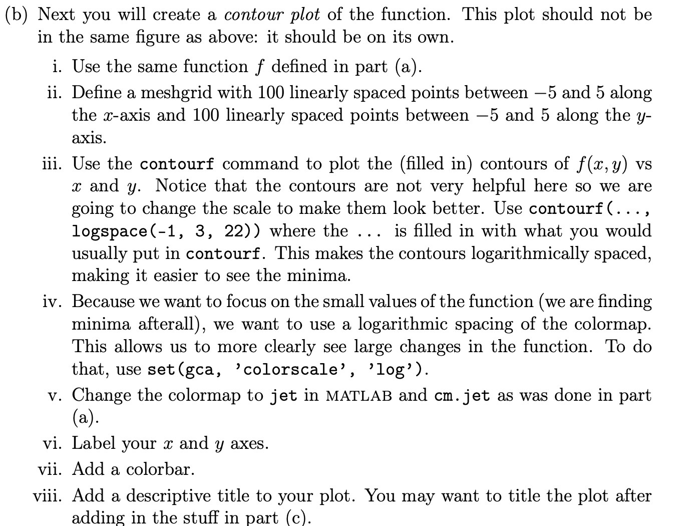
(b) Next you will create a contour plot of the function. This plot should not be in the same gure as above: it should be on its own. i. ii. iii. iv. vi. vii. viii. Use the same function f dened in part (a). Dene a meshgrid with 100 linearly spaced points between 5 and 5 along the maxis and 100 linearly spaced points between 5 and 5 along the y- axis. Use the contourf command to plot the (lled in) contours of f(a:,y) vs 33 and 3;. Notice that the contours are not very helpful here so we are going to change the scale to make them look better. Use contourf (. . . , logspace(1, 3, 22)) where the . . . is lled in with what you would usually put in contourf. This makes the contours logarithmically spaced, making it easier to see the minima. Because we want to focus on the small values of the function (we are nding minima afterall), we want to use a logarithmic spacing of the colormap. This allows us to more clearly see large changes in the function. To do that, use set(gca, 'colorscale' , 'log'). . Change the colormap to jet in MATLAB and cm. jet as was done in part (3)- Label your a: and y axes. Add a colorbar. Add a descriptive title to your plot. You may want to title the plot after adding in the stuff in part (c)