can I get step by step instructions on how to finish this (On Excel)? thank you

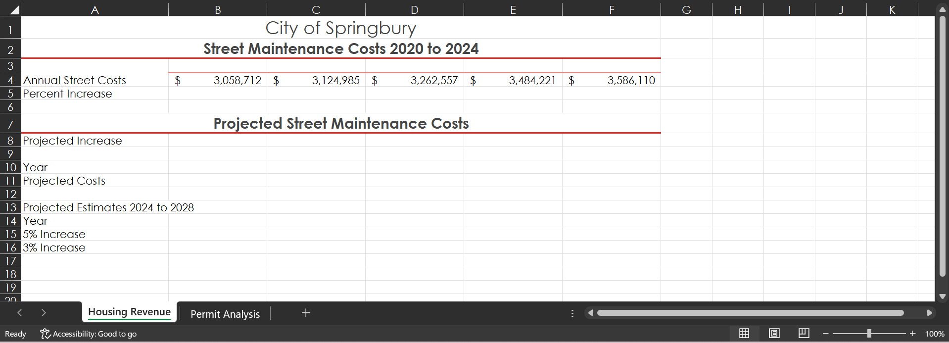
2	Change the Theme Colors to Orange. On the Housing Revenue sheet, in the range B3:F3, fill the year range with the values 2020 through 2024.
3	In cell C5, construct a formula to calculate the percent of increase in annual street maintenance costs from 2020 to 2021. Format the result with the Percent Style and then fill the formula through cell F5 to calculate the percent of increase in each year.
4	In the range B10:F10, use the fill handle to enter the years 2024 through 2028. Use Format Painter to apply the format from cell B3 to the range B10:F10.
5	Copy the value in cell F4 to cell B11. In cell B8, type 5% which is the projected increase estimated by the City financial analysts. To the range A8:B8, apply Bold and Italic.
6	In cell C11, construct a formula to calculate the annual projected street maintenance costs for the year 2025 after the projected increase of 5% is applied. Use absolute cell references as necessary. Fill the formula through cell F11, and then use Format Painter to copy the formatting from cell B11 to the range C11:F11
7	Use Format Painter to copy the format from cell A7 to cell A13. Copy the range B10:F10, and then Paste the selection to B14:F14.
8	Copy the range B11:F11 and then paste the Values & Number Formatting to the range B15:F15. Complete the Projected Estimates section of the worksheet by changing the Projected Increase in B8 to 3% and then copying and pasting the Values & Number Formatting to the appropriate range in the worksheet. Save your workbook.
9	Select rows 6:20, and then Insert the same number of blank rows as you selected. Clear Formatting from the inserted rows. By using the data in A4:F4, insert a Line with Markers chart in the worksheet. Move the chart so that its upper left corner is positioned in cell B7 and visually centered under the data above.
10	Display the Select Data Source dialog box, and then edit the Horizontal (Category) Axis Labels using the range that contains the years in B3:F3. Format the Bounds of the Vertical (Value) Axis so that the Minimum is 3000000 and the Major unit is 200000
11	Format the Chart Area with a Border by applying a Solid line. In the fifth column, click the last color. Change the Width of the border to 2 pt.
12	Click cell A1 to deselect the chart. Center the worksheet Horizontally, and then insert a Custom Footer in the left section with the file name.
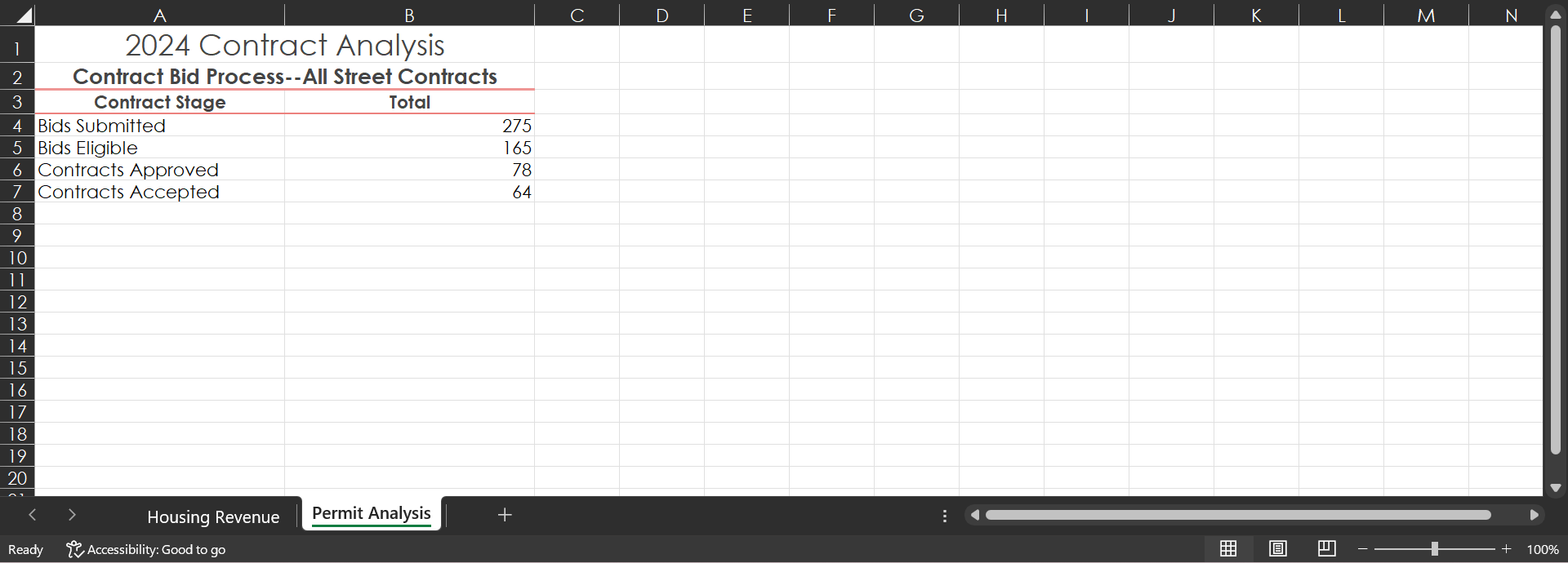
13	Display the Permit Analysis worksheet. Select the range A4:B7 and then insert a Funnel chart that depicts the number of bids in each stage of the bid process. Change the chart title to 2024 Contract Bids and then drag the chart so that the upper left corner aligns with the upper left corner of cell A10. Change the chart Height to 2 and the Width to 4.
14	Format the Chart Area with a Border by applying a Solid line. In the sixth column, click the first color. Change the Width of the border to 3 pt.
15	Deselect the chart, and then change the Orientation to Landscape. Center the worksheet Horizontally, and then insert a Custom Footer in the left section with the file name.

A B 2024 Contract Analysis Contract Bid Process--All Street Contracts Contract Stage Total Bids Submitted Bids Eligible Contracts Approved 275 Contracts Accepted 78 64 Housing Revenue Permit Analysis Ready Accessibility: Good to go